A new version of ObserVIEW (2025.1) is now available for download. In this latest software release, access a new random test generation option, STAG updates, improved file performance, and more.
Random Test Generation
FDS Combine
Create Field-correlated Test Profiles from Measured Data
The fatigue damage spectrum (FDS) in ObserVIEW displays the amount of fatigue damage a product will experience in a frequency range. For vibration testing, engineers can use the FDS to create a random test profile that is the damage equivalent to the recorded environment.
In ObserVIEW 2025.1, the Random Test Generation option allows engineers to create a profile from multiple channels or files. The result is a test encompassing some or all forms of potential fatigue. The VibrationVIEW control software supports these profiles, making it easy to navigate from analysis to testing.
To create FDS tests from multiple files, the engineer defines the lifetime cycle of the test item and the field environments it experiences within that cycle. A multiplier is assigned to each of the environments to simulate an equivalent overall lifetime usage target with correct amounts of fatigue damage from each. Engineers can set the test duration and confirm the acceptability of the accelerated profile with the ERS tolerance.
The Analysis Ranges feature of ObserVIEW makes it easy to add multiple test environments within a single project. Individual waveforms from each environment can be organized into groups for simpler processing. ObserVIEW also displays the statistics for each waveform.
Random Test Generation can be used as a visualization or test development tool. Engineers can graphically represent the relationship between environments or develop a test from them for product development.

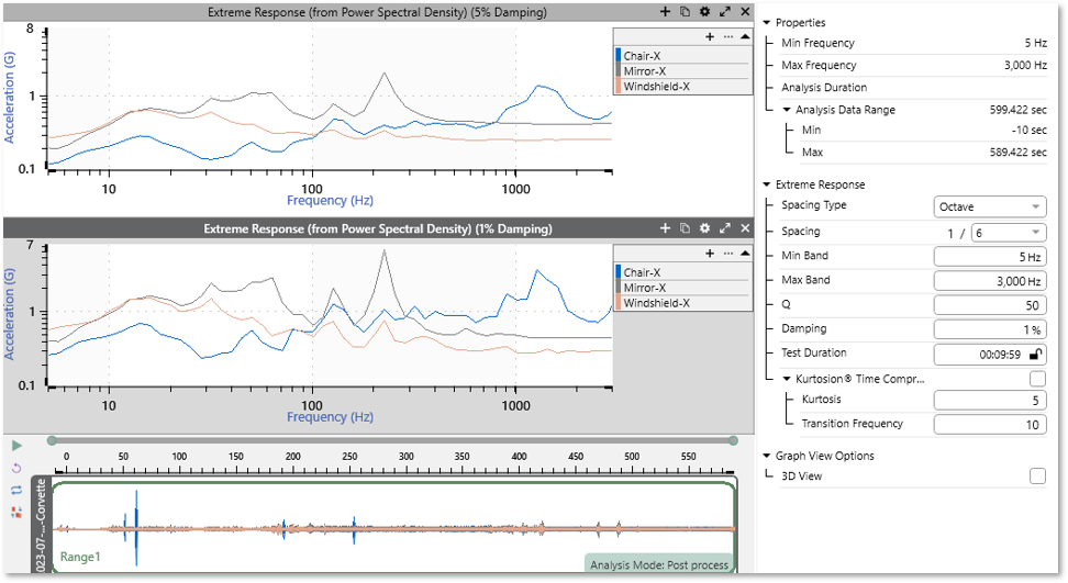
ERS: Extreme Response Spectrum
The ERS is a spectrum that represents the maximum amplitude response to random excitation. Engineers can use it as a tool to evaluate vibration severity between:
- Different field environments
- A field environment and test specification
- Different test specifications
ObserVIEW 2025.1 includes an ERS graph trace option. It works on any acceleration PSD data (FDS Test Spectrum, PSD, pasted trace, etc.). The software program calculates the ERS from the FDS Test Spectrum toolbar setting and applies the Q value from the SRS parameters.
Customers can plot the ERS to validate FDS test acceleration. ObserVIEW can process one or multiple PSD files to create a composite ERS.
Example Uses
- Determine if an FDS test profile is over-accelerated
- Upload many recordings to analyze, combine the results, and determine if the test is over-accelerated
- Compare the ERS of a PSD to other ERS or SRS traces to calculate the SRS or maximax response spectrum (MRS)
STAG Updates
Compute FDS from Random Background Vibration in STAG
Sine Tracking, Analysis and Generation (STAG) is a tool for generating sine-on-random test profiles using field recordings. It separates rotational content from background random vibration, processing the sine and random content separately before generating a single test profile.
The first iteration of STAG exported the background random vibration to the VibrationVIEW software to generate an FDS, requiring both ObserVIEW and VibrationVIEW licenses. ObserVIEW 2025.1 can compute an FDS from random vibration, performing all processes within one software program. This improvement streamlines the test generation process.
Generate a Reference RPM Trace
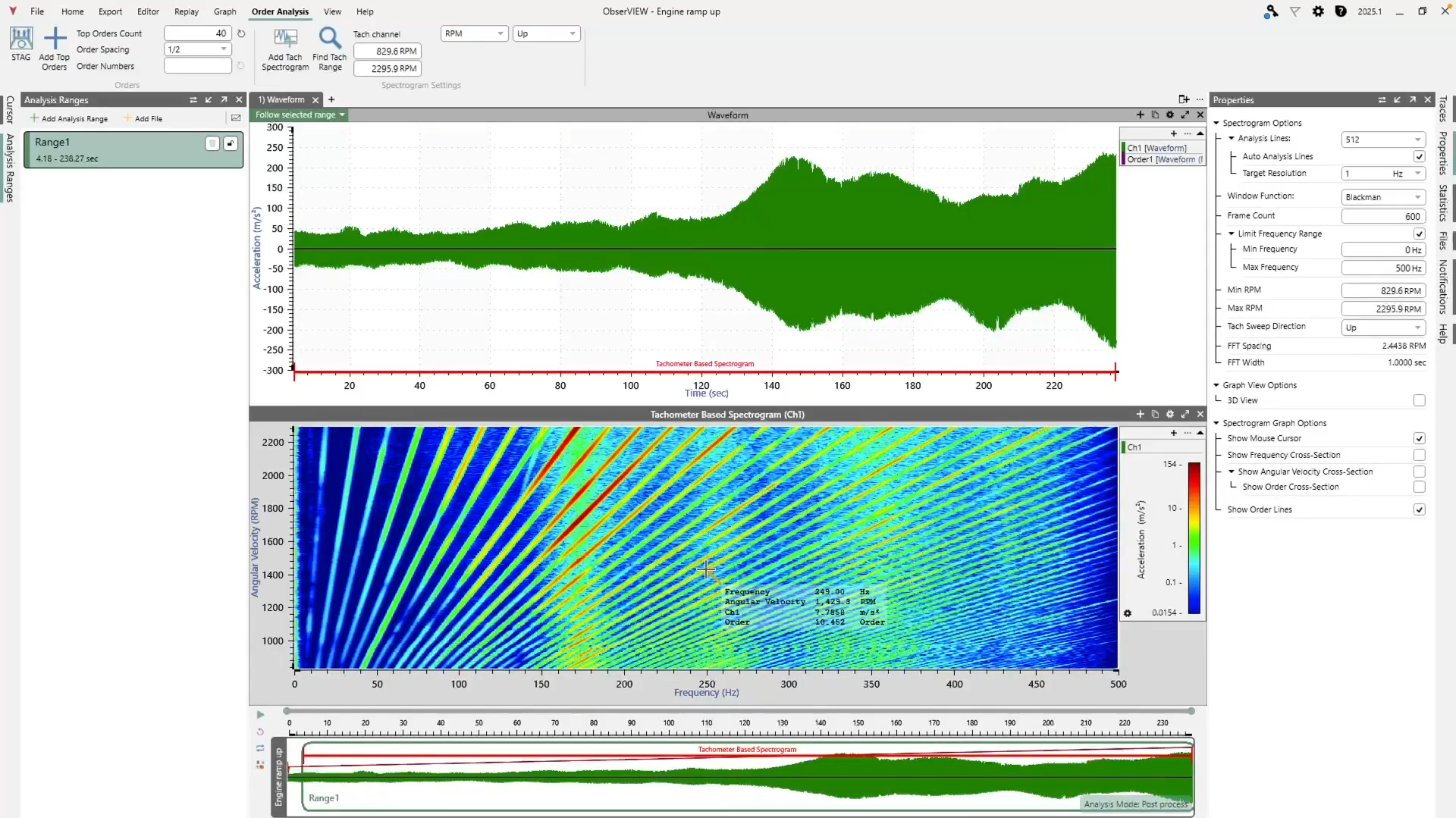
STAG uses an RPM reference trace and sensor data to separate the rotational content from the background random vibration and extract orders of interest. ObserVIEW 2025 makes it easy to generate an RPM trace if an RPM recording is insufficient or not possible.
For example, an engineer wanted to create a sine-on-random test for an engine of an agricultural machine. They recorded the engine as the throttle gradually increased the RPM. However, the recording of the RPM was insufficient. In a time spectrogram, the engineer could see consistently sweeping tones of various orders stacked on top of one another. They could select several points in the spectrogram and use math to generate a tone, but there were several points in the test where they wanted to slow down the RPM sweep and get a more detailed picture of the engine’s behavior.
In ObserVIEW 2025.1, the engineer can extract an RPM trace by marking the points where the first order’s RPM/time shifts on a time spectrogram and generating an RPM/time math channel approximation from those points. Then, they can create a trace with the new bandpass tracking filter math function with reference to the RPM/time approximation. The bandpass filter trace removes outside noise, making it easier to run the frequency tracking and producing a better RPM/frequency trace.
This workaround allows the engineer to generate a sine-on-random profile in STAG and reproduce the measured conditions without recording the engine RPM.
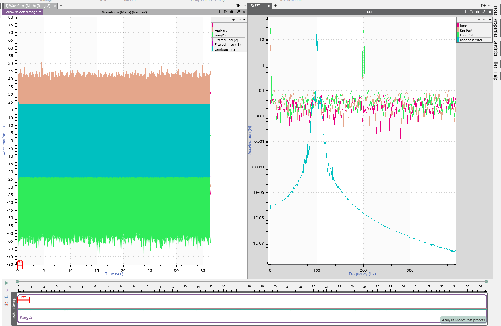
Bandpass Tracking Filter Math Function
A bandpass tracking filter math function was added to support the improvements in STAG, but it is useful for other applications, such as sine data reduction. This math function filters the input using a bandpass filter and a defined frequency.
For example, trackingbandpass(“Ch1”, “Frequency”, 0.1, 15) applies a bandpass filter to Ch1 with a 0.1 fractional bandwidth and a maximum bandwidth of 15.
Bandpass filters help isolate frequency bands of interest, often attenuating high-frequency noise so that other vibration behavior is visible.
- Bandpass around a spectrogram trace to get a filtered order trace
- Remove order tones from raw time data
Improved Large File Performance (100+ GB)
Engineers in industries with oversized test items, such as energy pipelines, may record extremely large files from the field.
Improvements have been made in ObserVIEW 2025.1 to improve the processing of large recording files, helping engineers get their data on the screen quicker—and with less RAM—than before.
Reference Multiple Data Ranges in a Math Traces Equation
ObserVIEW 2024 introduced Analysis Ranges, where users can add multiple analysis ranges to a project and easily navigate between them. In 2025.1, the Math Traces feature supports equations with multiple data ranges.
To specify an analysis range, include a tilde symbol (~) after the channel and denote the range as a, b, c, etc. Math Traces can reference a graph trace, a global math trace, or a pasted trace.
For example, the following equation calculates a channel’s total fatigue damage for two data ranges:
sum(fds(v1~a), fds(v1~b))
Where v1 is Channel 1, a is Range A, and b is Range B.
Floating License Support
ObserVIEW 2025 includes a “floating license” mode for more convenient software management. This license is one shared key for a specified number of concurrent users accessing any PC on the same network. Individual access resets after 24 hours of inactivity with the server, returning to the shared license pool for other users to access.
This option allows organizations to optimize software usage across multiple users without purchasing individual licenses for each workstation. With floating license support, team members can access the software from any workstation, allowing for flexible work arrangements and ensuring critical tasks can continue even when specific computers are unavailable.
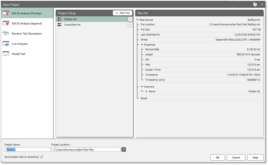
Multiple Waveform File Support
The Analysis Ranges pane in ObserVIEW allows users to add multiple analysis ranges to a project and easily navigate between them rather than create a new project for each data range of significance. In version 2025.1, the Analysis Ranges pane includes an Add File option, where users can analyze multiple waveform files in the same project and overlay/combine spectrums. It is also accessible when creating a new project and in Random Test Generation.
For example, say an engineer is analyzing two similar manufacturing machines; one jams occasionally, and the other is functional. The engineer hypothesizes that the cause is a mechanical timing issue and wants to compare the functional machine against the non-functional one. They record each machine separately and then use ObserVIEW to identify the difference in timing between mechanical events. The engineer identifies an event that appears to occur too early, guiding them to the malfunctioning component.
Change Between Projections of Complex Data
Engineers often use different complex data visualizations to identify relationships in the data. This release has made switching between projections of complex data in ObserVIEW more efficient.
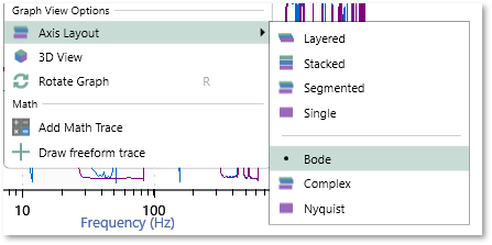 Customers can now select complex layouts from the Graph View Options: Bode, Complex, and Layered. These options are available for any graph with complex data, including transfer function, coherence, and cross-spectral density graphs. To access them, right-click on the graph and navigate to Axis Layout.
Support for Shock Recordings with Negative Time Data
In shock testing, time zero is at the shock event’s trigger. However, data files from shock tests may have negative time data due to pre-event recording. Engineers might record this data to capture baseline behavior or early transients, verify sensor stability, or check for noise.
ObserVIEW 2025 supports negative time data for TXT, CSV, and UFF files, including an offset for negative time data. Engineers can import text files and view T=0 at the time of the event trigger, aligning with the view in the control software.
ObserVIEW will continue to support negative time data for VFW files that have a pre-trigger and are recorded in autonomous mode or Live Analyzer.
Additional Features
- Move satellite maps from Bing to Azure
- Date/time axis and PDF graphs out of feature preview
- New Math functions
- Chinese Help file translation