The purpose of sine testing is to expose the device under test (DUT) to a single-frequency sine tone at a defined amplitude (a “pure tone”) and for a defined time. When running a sine test, the system monitors the control signal’s amplitude at the demand frequency, which ideally should be a replication of the pure tone on the shaker table.
Due to the nature of shaker systems, controllers will pick up contributions from noise and harmonics in addition to the pure tone. This background noise may alter the control reading, prompting the system to adjust the drive signal.
Sine tracking filters isolate the pure sine tone from noise/harmonics outside the center frequency. They allow the controller and engineer to read the amplitude at the center frequency and ensure the test is controlled properly.
Theoretical Example
Suppose we run a sine sweep from 5Hz to 100Hz with a 1G acceleration. As the sweep advances, let’s figuratively pause at 10Hz. At 10Hz (the center frequency), the drive outputs 1G, but the input is acquiring noise from the other frequencies (5Hz, 20Hz, 50Hz, 100Hz, etc).
Let’s say there is a harmonic at 100Hz contributing 0.5G and system noise at 50Hz contributing 0.3G. The controller concludes there is an acceleration of 0.8G at 10Hz. It adjusts the drive to account for the reading at 10Hz and outputs the remaining 0.2G required to reach 1G at 10Hz.
The controller now measures a total of 1G at 10Hz. However, it is not outputting 1G at 10Hz but 0.2G. The drive has changed significantly, and the test is not producing the desired results.
Sine Tracking Filters
A sine tracking filter isolates the pure sine tone so the controller can read its amplitude and control the test correctly. It is called a tracking filter because it tracks the center frequency as the test sweeps through the test’s frequency range and filters out noise at frequencies outside of the center frequency. Without a tracking filter, the controller assumes all the energy the test generates relates to the test’s entire frequency bandwidth because controllers assume a perfect scenario.
In the previous example, acceleration readings at frequencies other than 10Hz affected the test. If we apply a sine tracking filter, the controller can filter out the noise at 100Hz (0.5G) and 50Hz (0.3G).
Tracking Filters Experiment
The previous theoretical example provided a simple explanation to demonstrate how frequencies of non-interest can affect control readings. In reality, the vibration controller makes adjustments based on the average root-mean-square (RMS) of the frequency bandwidth. The following experiment will provide a more in-depth explanation.
Setup
We set up a sine sweep from 300Hz to 4,000Hz at 1G and looped the output to the input. We also connected an ObserVR1000 to input Channel 2 and generated a 1,000Hz wave at 1G acceleration in Live Analyzer.
Without Tracking Filter
Figure 1. Sine sweep, no tracking filter.
As the controller sweeps through each frequency, it calculates the average RMS for the entire bandwidth (300 to 4,000Hz), not just the frequency of interest (Figure 1). The 1,000Hz noise contributes to the average RMS value outside of the 1,000Hz range and thus affects the control reading. The acceleration from noise and harmonics doesn’t belong to the control, but the controller averages all unfiltered contributions into the control.
With Tracking Filter
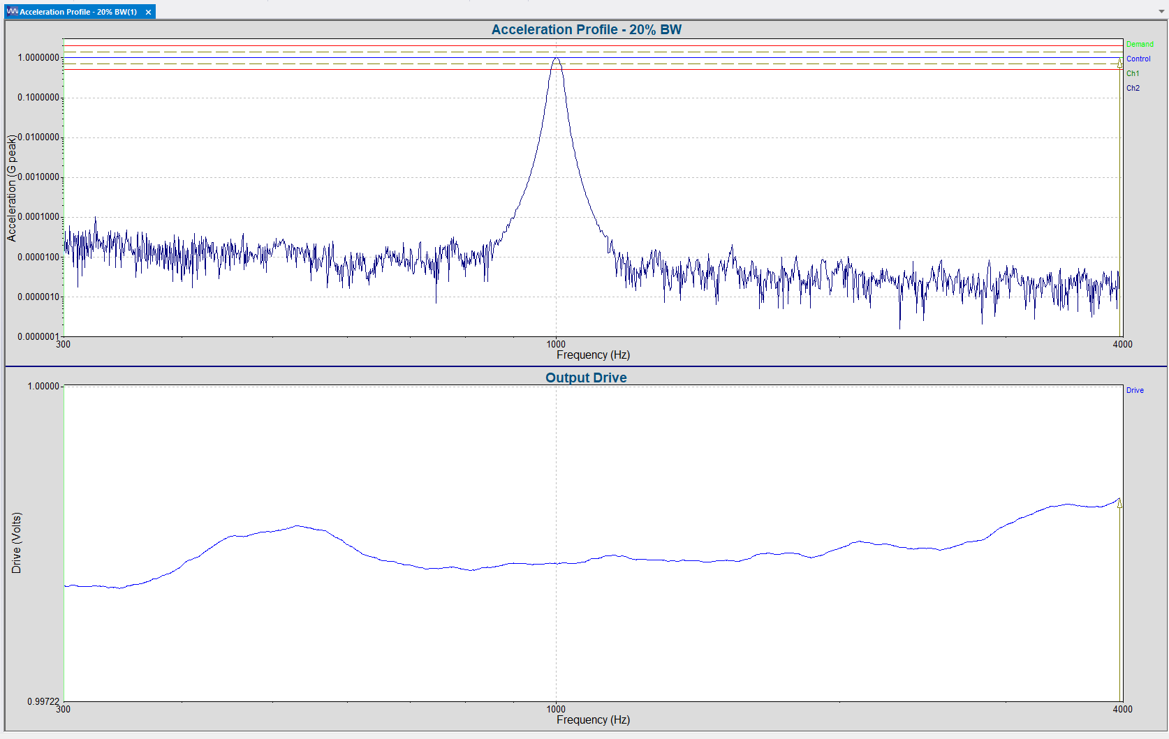
Figure 2. Shape of a 20% bandwidth tracking filter.
With a tracking filter, we can reduce the bandwidth of the RMS average. This action allows the controller to pass through less noise. Figure 2 shows the shape of a tracking filter with a 20% bandwidth.
In VibrationVIEW‘s Sine software, the user defines the bandwidth of the tracking filter. The tracking filter bandwidth is defined as both a fractional and maximum bandwidth.
A fractional bandwidth sets the bandwidth of the tracking filter as a percentage of the drive frequency. For example, consider a 20% fractional bandwidth. When the sine sweep (drive frequency) is at 10Hz, the tracking filter bandwidth is 20% of 10Hz or 2Hz. With a 2Hz tracking filter bandwidth and at a 10Hz drive frequency, the control averages the RMS values from 9Hz to 11Hz and filters out all other frequencies.
The fractional bandwidth increases as the drive frequency increases. For example, at 10Hz, a 20% fractional bandwidth is 2Hz. At 2,000Hz, however, the fractional bandwidth is 400Hz. At this frequency, noise between 1,800Hz and 2,200Hz could contribute to the reading.
The maximum bandwidth sets the maximum allowable bandwidth of the tracking filter. The fractional bandwidth cannot exceed the maximum bandwidth, and the controller always uses the smaller of the two.
When a sweep begins at a low frequency, the fractional bandwidth increases until it equals the maximum bandwidth. This point is called the crossover frequency. After the test reaches the crossover frequency, the maximum bandwidth governs the tracking filter bandwidth.
Example
Figure 3. The behavior of a tracking filter at various fractional bandwidths.
As an experiment, we set various fractional bandwidths for our tracking filter and observed the tracking filter’s behavior at 1,000Hz.
As the filter swept up, the wider tracking filters encountered the 1,000Hz input signal sooner than the narrower tracking filters (lower bandwidth percentage). The higher the fractional bandwidth percentage, the wider the tracking filter. The wider the tracking filter is, the earlier the acceleration will increase.
In Figure 3, the acceleration increases quickest with the highest (20%) fractional bandwidth percentage. The rise in acceleration occurs much closer to 1,000Hz when using the narrowest fractional bandwidth percentage (1%).
Final Comments
-
- Smaller value tracking filters (narrower bandwidths) provide increased filtering and greater stability
- Stability can improve performance when sweeping through sharp resonances
- Reduced filtering (larger bandwidths) will improve performance at extremely low frequencies
- Increased filtering comes at the cost of increased response times, which requires more measurement time
- Tracking filter response time and bandwidth are inversely proportional. Although one can set a response time and a tracking filter bandwidth, performance is limited by this inverse relationship. 1/TFBW = minimum RT in seconds and 1/RT = narrowest TFBW