We often receive questions related to designing products that are robust against vibration inputs from either the end-use environment in which the product must function or the operational vibration. Previous resources have detailed the processes of developing appropriate vibration tests using the fatigue damage spectrum (FDS) and other methods but less about mitigating the problem early in the product development cycle.
This resource discusses a design-for-reliability concept called the factor of 2 rule: a guideline for avoiding resonance-related failures. It introduces the factor of 2 rule, discusses why it works, and includes several examples.
Instead of reading this article, you can view the tech talk.
Avoiding Resonance in Design
Resonance occurs when a component’s natural frequency matches the frequency of an external vibration or forcing function. This equivalency leads to a maximum energy transfer between the environment and the product, resulting in large oscillations and excessively high stress amplitudes. With nowhere for the energy to go, the fatigue accumulates rapidly, and the product eventually fails.
This phenomenon can occur in machine bracketry, circuit cards mounted in aircraft, structures subjected to wind and earthquakes, and any other applications where unavoidable operational forces are present. Fortunately, there are steps in the design phase of product development that can help avoid failures due to resonance.
Factor of 2 Rule
Resonance leads to excessive accumulation of fatigue damage and potential mechanical failure. A good engineering practice is to confirm that a component’s resonant frequencies are at least a factor of 2 above/below operational frequencies. This rule is called the “factor of 2.”
Damping
Another critical consideration in product design is damping. A component can be critically damped, overdamped, or underdamped.
- Critically damped: The system returns to equilibrium as quickly as possible without oscillating.
- Overdamped: The system returns to equilibrium slowly without oscillating.
- Underdamped: The system oscillates with decreasing amplitude if there is no excitation, but it can resonate–and potentially become unstable with catastrophic consequences–if excited at its natural frequency.
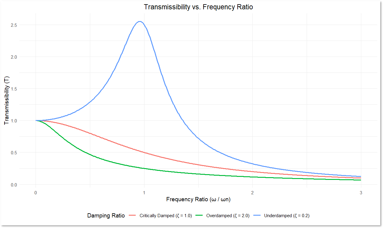
Frequency ratio (frequency over natural frequency) of critically damped, overdamped, and underdamped structures.
To avoid over-amplification (even when underdamped), a component’s resonant frequencies must be separated from the system’s operational vibration inputs.
When the natural frequency, ωn, is at least a factor of 2 away from the system’s response, it significantly reduces the amplitude and the potential for rapid accumulation of fatigue and failure.
Damping is present in real-world systems and reduces the amplitude of resonant vibrations. However, if the natural frequency is close to the environmental frequency–even with damping–the system can still experience significant vibration. When the natural frequency has at least a factor of 2 separation from any environmental inputs, it reduces the risk of mechanical failure.
Quality Factor
Most systems have some level of damping. The quality factor, Q, of a resonant system is approximately inversely proportional to the damping ratio, ζ, as Q=1/2ζ . High-Q systems (low damping) are more susceptible to the effects of resonance.
The factor of 2 rule is a conservative guideline to ensure that the risk of resonance is minimized, even in lightly damped systems.
Underdamped (ζ<1) Examples
-
- Car suspension systems: When a car runs over a bump, the suspension system (composed of springs and dampers) allows the car to oscillate several times before coming to rest. This behavior balances comfort (less oscillation) and stabilization.
- Guitar strings: When a musician plucks a guitar string, the string vibrates, producing sound waves that gradually diminish in amplitude due to air resistance and internal friction, exhibiting underdamped behavior.
- Mechanical clocks: The pendulum in a mechanical clock oscillates with underdamped motion, where the damping force is low enough to allow continued oscillations but significant enough to eventually bring the pendulum to rest.
Critically damped (ζ=1) Examples
-
- Automotive shock absorbers: Engineers design shock absorbers to quickly return the vehicle to a stable state without oscillation after a disturbance. This behavior ensures a smooth ride and quick stabilization.
- Door closers: Closers are the mechanism that ensures a door closes smoothly and quickly without bouncing back. The door closes at a constant rate and settles into the closed position without oscillation.
- Camera stabilizers: High-end camera stabilizers use critically damped systems to minimize shaking and quickly stabilize the camera after movement for smooth footage.
Overdamped (ζ>1) Examples
-
- Heavy door closers: Heavy industrial or vault doors with strong closing mechanisms return to the closed position slowly, steadily, and without bouncing.
- Electronic filters: Certain low-pass electronic filters designed to remove high-frequency noise from signals may be overdamped, resulting in slower response times to changes in the input signal.
- Seismograph mechanisms: Instruments that measure earth tremors or vibrations are often overdamped to avoid oscillations that could distort the measurements. The overdamped mechanism ensures the recording needle returns to its original position slowly and without oscillation.
Finite Element Analysis
Engineers can use finite element analysis (FEA) to simulate and analyze vibration before manufacturing. This step is performed early in the product development cycle. FEA results should be confirmed on prototype hardware to confirm the accuracy of boundary conditions, thermal effects, and material properties.
Vibration Research offers several options for performing resonance searches and validating analytical models. These analyses and confirmations are necessary to perform on the product and any test fixtures for vibration testing. A vibration test fixture that imparts undesired resonant energy into a product will cause ambiguous test results and must be avoided.
After finalizing the design and confirming the analytical models, the engineer moves to production-intent parts with a representative vibration test.
Frequency Response Function
A system’s response to a dynamic load is characterized by its frequency response function (FRF). The FRF is a mathematical tool that describes how a system responds to input frequencies. It shows the relationship between the input frequency and output amplitude and phase, indicating how effectively the system transmits different frequencies. The response is significantly higher when closer to the natural frequency.
Vibration Modes
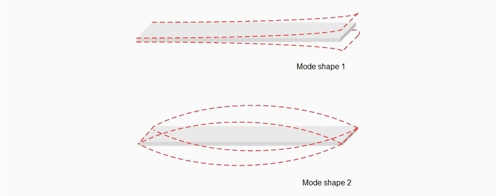
In a vibrating system, energy is distributed among various modes: the characteristic patterns of motion that a system undergoes when it vibrates at specific frequencies. Each mode is associated with a particular natural frequency, and the shapes of these patterns are called mode shapes.
For example, a beam’s first mode can be a simple bending shape, the second a double-bend shape, and so on. Each mode shape corresponds to a higher natural frequency as the mode number increases.
Factor of 2 Rule
A factor of 2 separation protects a product from the primary resonance, or first mode, and its harmonics, preventing system excitation into rapid failure. As an example, let’s consider an aircraft wing design. If the wing’s natural frequency is 20Hz, a factor of 2 separation would suggest avoiding operational and environmental frequencies between 10Hz and 40Hz. This separation would help prevent resonance from aerodynamic forces and engine vibrations, ensuring structural integrity and safety.
Typically, vibration sources are wideband inputs and not purely sinusoidal. Sources can include a range of frequencies due to various operational sources and background noise. The factor of 2 rule is conservative and accounts for a broad frequency range.
The factor of 2 rule balances the complexity of exact calculations with the need for a straightforward design principle to ensure reliable performance in varying conditions. This conservative approach of maintaining a natural frequency that is at least half/twice the frequency of operational inputs ensures that products will pass vibration testing and survive in the end-use environment.
Math of Factor of 2 Rule
The FRF is fundamental to the explanation of the factor of 2. An FRF describes how a system responds to an input signal at different frequencies. It provides information about the system’s amplitude and phase response.
An FRF shows how the output amplitude varies with frequency. The FRF function can be derived from the equation of motion and includes a forcing function, F0, mass, natural frequency (ωn), damping factor (ζ), and frequency (ω).
The FRF is related to transmissibility in that transmissibility is the ratio of the output response to the input response at a particular frequency. An FRF provides the necessary data to calculate transmissibility.
Figure 1 is a transfer function graph in the ObserVIEW software. In ObserVIEW, transfer function graphs are essentially equivalent to FRF graphs, as the transfer function is based on measured data like the frequency response function.
Figure 1. Transfer function graph in the ObserVIEW analysis software program.
These graphs show the measured response of a system in terms of magnitude and phase across a range of frequencies. As such, they provide a practical representation of the system’s behavior under real-world conditions, capturing any nonlinearities and noise in the measurements. They are a good starting point for understanding how well the factor of 2 rule applies to a system.
Damped Harmonic Oscillator Response
Let’s look at a basic equation of motion and relate it to the FRF.
Consider the equation of motion for a damped harmonic oscillator with displacement response x(t) to a periodic force F(t)=F0(cosωt):
(1) 
Where m is the mass of the system, c is the damping coefficient, k is the stiffness, and ω is the forcing frequency.
The solution to the differential equation involves the system’s natural frequency…
(2) 
…and the damping ratio:
(3) 
The result is that the steady-state amplitude, X(ω), of the displacement is given by the frequency response function:
(4) 
Note: When the forcing frequency, ω, approaches the natural frequency, ωn, the denominator of X(ω) decreases, leading to a large amplitude response. This phenomenon is resonance.
The peak response occurs at a frequency…
(5) 
…close to ωn for small damping (ζ<<1).
Numerical Example
Using the frequency response function:
(6) 
We note that at resonance:
(7) 
And, when ω=2ωn with ζ=0.05, we find:
(8) 
(9) 
(10) 
For a typical lightly damped system, ζ is small, and the amplitude at 2ωn is much smaller than the amplitude at ωn, demonstrating the effectiveness of the factor of 2 rule.
The numerical result shows that at twice the natural frequency, the response amplitude is only about 3.3% of the amplitude at resonance. This significant reduction illustrates the usefulness of the factor of 2 rule. Designing the system to have a natural frequency at least a factor of 2 away from any dominant environmental frequency substantially reduces the risk of excessive vibrations due to resonance.
Amplitude Reduction
More generally, since Q and ζ have an inverse equivalence, we can express the amplitude reduction factor in terms of either quality factor or damping ratio.
(11) 
Since  then
then 
(12) 
Automotive Example
Automotive engine order frequencies are harmonics of the engine’s rotational speed and firing frequency, which varies with the number of cylinders and the type of engine cycle (2-cycle, 4-cycle, etc.).
Consider a 4-cylinder automotive engine that idles at 800 RPM, generally operates at 2,000 RPM, and has intermittent peaks at 3,500 RPM. A 4-cylinder automotive engine fires twice per revolution, so the dominant vibration input is second order.
For our example, this translates to:
Idle:
(13) 
General operation:
(14) 
Intermittent operation:
(15) 
By the factor of 2 rule, we should design any components influenced by engine vibration to have resonant frequencies > 234Hz.
Circuit Card Example
One area of design focused on robustness against resonant frequencies is large circuit card assemblies used for inverters and other power electronics found in battery electric vehicles and marine and aircraft applications.
Without understanding these systems’ operational environments and modes, it is not unusual for large circuit board assemblies to have natural frequencies that cause large components, such as capacitors or inductors, to fatigue and fall off. Engineers must use analytical methods to predict these systems’ modes, verify them in the lab, and adjust the design if necessary to ensure that resonant frequencies are at least a factor of 2 above the harsh vibration environment they must survive.
There are several ways to adjust circuit card designs to ensure that resonant frequencies are out of harm’s way, including:
- Increasing the board stiffness with thicker materials
- Optimizing the board layout to distribute mass evenly and reduce the overall weight
- Securing large components with SilGel encapsulation or special cage support structures
- Using FEA to predict resonant frequencies and to ensure that the factor of 2 rule is applied
- Performing resonance searches on hardware to confirm models
- Validating designs with vibration testing using FDS-correlated profiles
Example
Figure 2 shows Gaussian noise with a 90Hz resonance and a 1g, 200Hz sine wave.
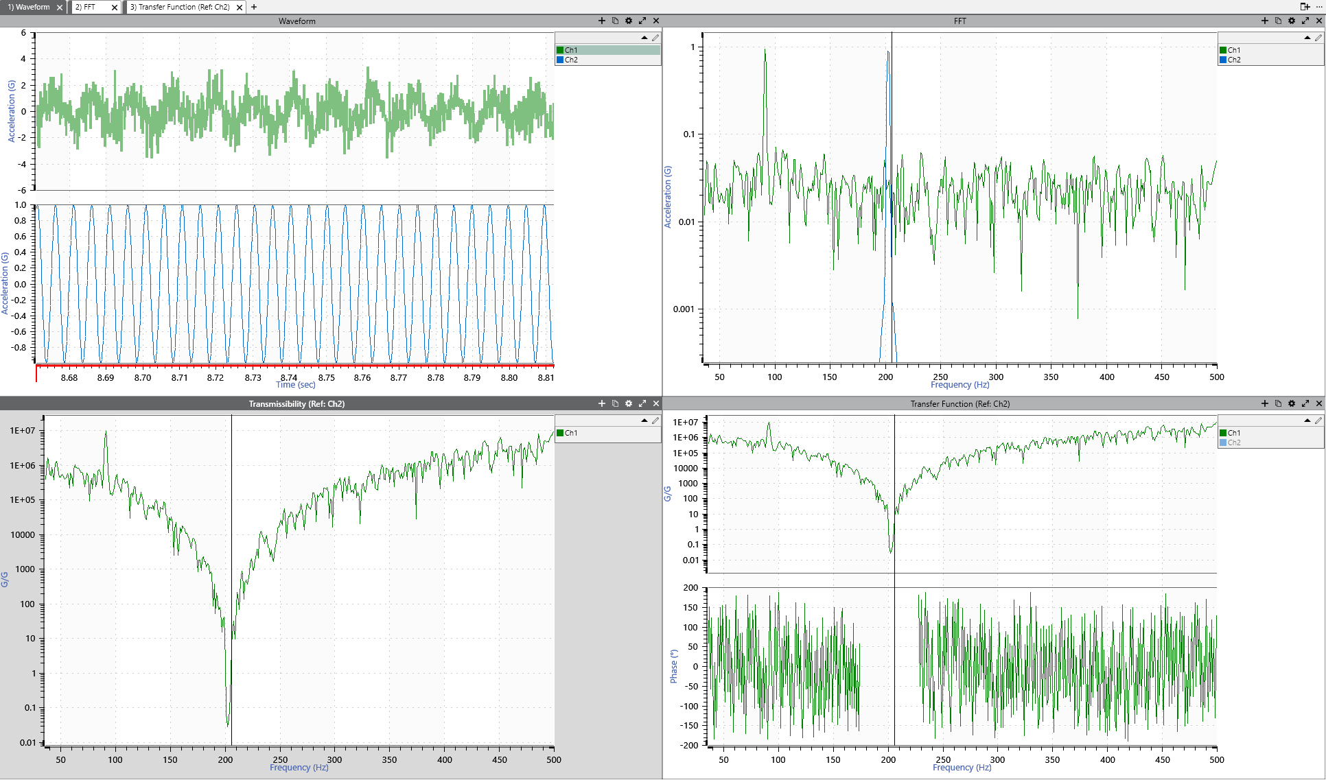
Figure 2. Gaussian noise and a sine wave.
Figure 3 shows the acceleration waveform converted into a displacement waveform.
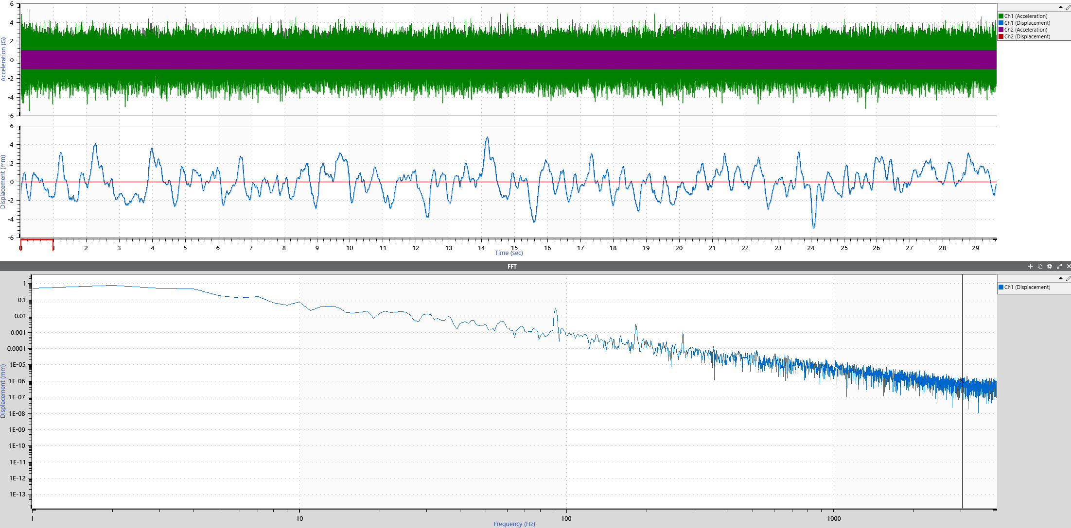
Figure 3. Displacement waveform from the Gaussian noise acceleration waveform.
Referring to the FFT, there is about 0.014796mm displacement at 90Hz and 0.000384mm displacement at 180Hz. This amplitude reduction is about 0.0259, which the idealized factor of 2 rule predicted previously.
Conclusions
While the factor of 2 rule isn’t derived from a single mathematical theorem, it aligns with the understanding of resonance, frequency response, and the impact of damping on system behavior. It provides a practical safety margin to ensure reliable operation away from resonant frequencies, thereby preventing excessive vibration and potential failure in real-world applications.
- Be aware of the end-use environment amplitude, frequency content, and design life requirements. Use this information to design resonance-resistant products and develop vibration profiles based on correlated fatigue damage spectrum method.
- Design critical components such that resonance is separated by a factor of 2 from vibration drivers.
- Use the appropriate Q when performing analyses. As Q increases, the factor of 2 rule has more forgiveness.
- Confirm FEA with the Sine Resonance Track and Dwell functionality.
- Validate design with an FDS-correlated profile or required standard. Remember to confirm resonant characteristics of vibration test fixtures.