Signal analyzers use the fast Fourier transform (FFT) to compute the power spectral density (PSD) of a Gaussian-distributed random waveform. The FFT is a linear transform, and the input is Gaussian. As a result, the output of the FFT at each frequency line is a complex number with a Gaussian real part and a Gaussian imaginary part. The analyzer squares these values and adds them to get the magnitude. As such, the square magnitude of the FFT output is a Chi-squared distributed random variable with 2 degrees of freedom (DOF).
To compute an averaged random PSD, the analyzer:
- Measures F frames of time data,
- Calculates an FFT of each frame, and
- Averages the square magnitudes
As a result, the averaged PSD of a Gaussian waveform is a Chi-squared distributed random variable with (2*F) DOF. This is where the DOF averaging specification for a random vibration test comes from.
In a practical sense, we can directly compute confidence intervals and probabilities from the equations defining the Chi-squared distribution. The Chi-squared distribution with n degrees-of-freedom has a probability density function and cumulative distribution function as follows.
PDF:
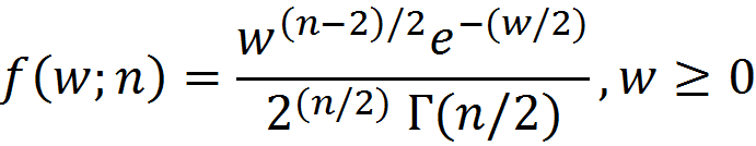
CDF:
![]()
Where Γa is the gamma function, and P(x,a) is the regularized lower incomplete gamma function.
Tolerance Bands
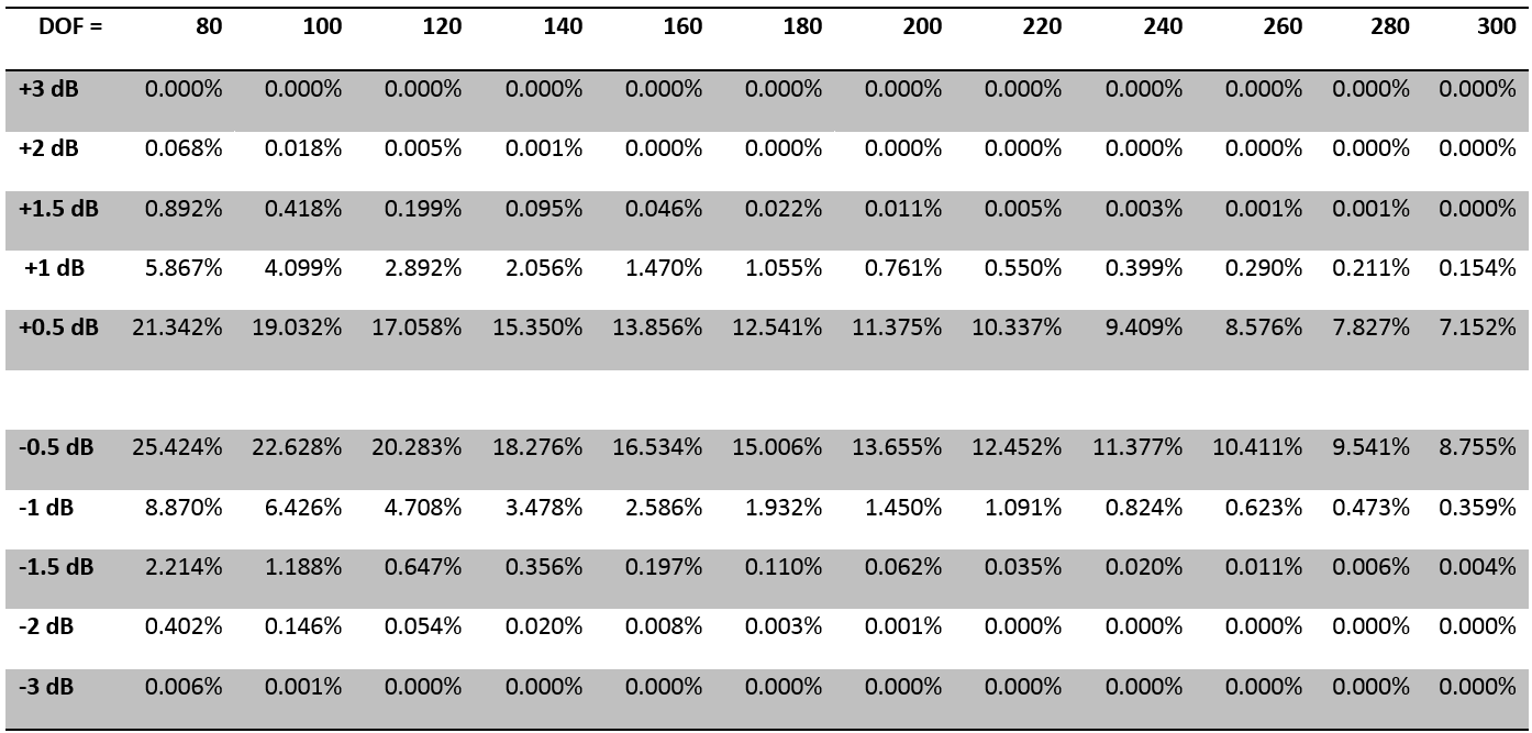
Using this relationship and given a DOF value, we can tabulate the probability of exceeding a given dB level from the mean. If we note that the mean of a Chi-squared random variable is equal to the DOF, n, then, using MATLAB® notation,
Pr[x<dB] = gammainc(10^(dB/10)*DOF/2,DOF/2,’lower’) for dB<0
Pr[x>dB] = gammainc(10^(dB/10)*DOF/2,DOF/2,’upper’) for dB>0
Table 1: Probability of a PSD value exceeding the tolerance dB for a given DOF
Compounded Probability
The probability calculations give the probability of a single line being outside the tolerance band. The typical random test is composed of a broad band of frequencies, with 200, 400, 800, or more lines distributed over that band, and we are interested in knowing the probability of any one of those lines going outside of the tolerance or abort bands. To account for this we assume the lines are independent, and compute the probability for having all lines within the specified tolerance band. This is done by computing the probability of a single line being within the tolerance range, and then combining this probability with all other lines. Mathematically this is done by multiplying the probabilities together, so for a given number of lines we can tabulate the probability of meeting the tolerance using the formula pl where p is the probability of a single line being in-tolerance, and l is the number of lines.
This calculation tells us what DOF parameter is required to achieve and maintain a stated tolerance with reasonable probability. Since the waveform is random, we can never achieve a full 100%, but some cases get very close.
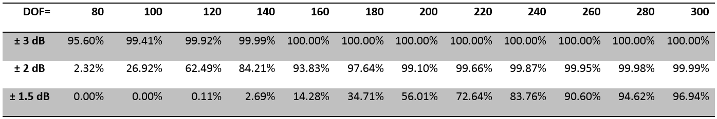
Table 2: Probability of all lines within tolerance band, 800 lines
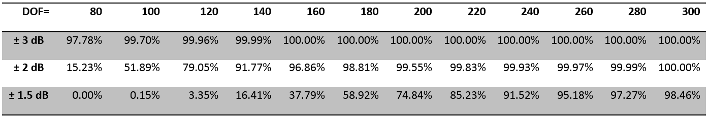
Table 3: Probability of all lines within tolerance band, 400 lines
Confidence Intervals
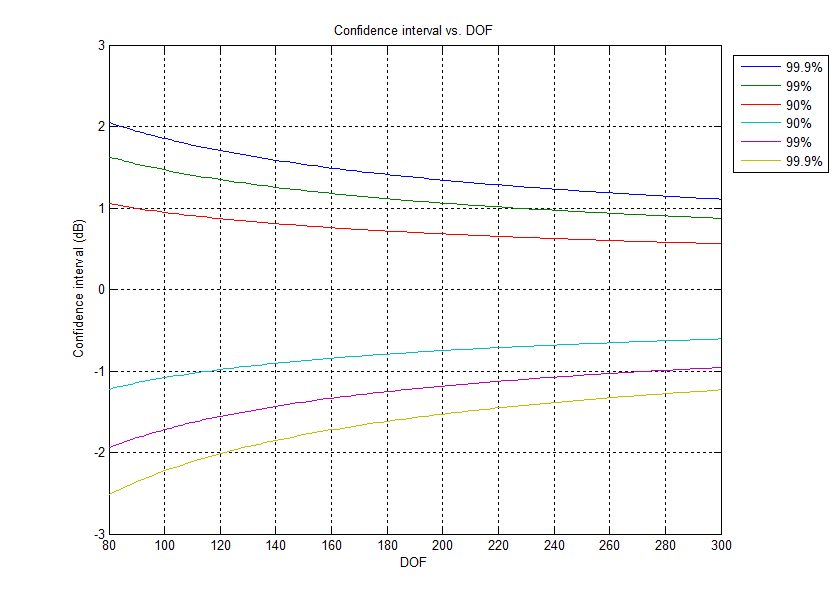
This calculation can be reversed, and we can also compute the dB levels given a probability value. This is typically expressed as a 90%, 99%, or 99.9% confidence interval. The 90% confidence interval gives the range of dB values which cover the central 90% of the probability curve. In other words, there is a 5% probability of being less than the lower bound, and a 5% probability of being greater than the upper bound, and a 90% probability of being within the stated bounds. These confidence intervals can be tabulated and plotted as a function of DOF.
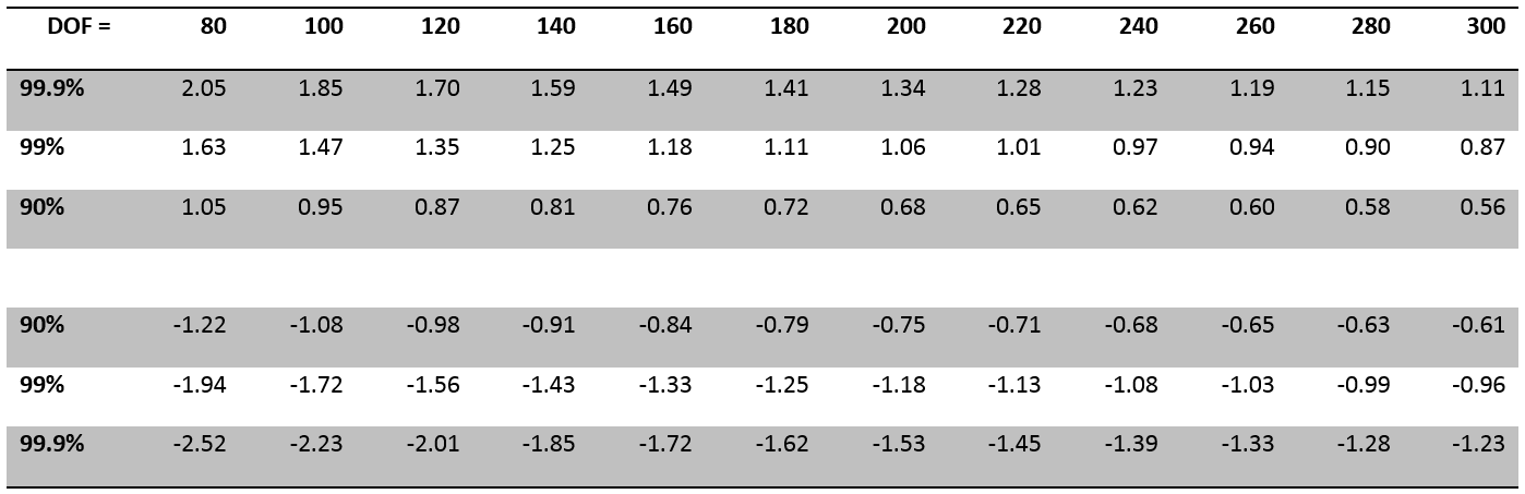
Table 4: Confidence interval, in dB, of a PSD value for a given DOF
Windowing and Overlap
The above calculations, with DOF equal to 2 times the number of frames, assume independent frames of data. When overlapping frames and window functions are used, the frames are no longer independent, and the effective DOF of the average will not be simply a multiple of the number of frames. The effective DOF can be estimated numerically by simulating data with the specified overlap and window function applied, computing the statistics of the resulting PDF, and comparing those statistics to a Chi-squared distribution with a known DOF.
As a rule of thumb, for 50% overlap, and with a window function, you still achieve a DOF of nearly 2 times the number of frames averaged together. For 75% overlap you achieve a DOF of about 1 times the number of frames. The practical result is that for a given time interval you can double the effective DOF by using 50% overlap.