This paper originally appeared in Sound & Vibration, Volume 46, Issue 2, February 2012, pp. 9-12.
When selecting a vibration test type, test engineers typically have the most difficulty establishing the differences between sinusoidal vibration (sine testing) and random vibration testing. Sine testing helps describe how a structure vibrates naturally. Random vibration testing brings a device under test (DUT) to failure using vibration reflective of real life.

Figure 1. A sinusoidal waveform. Note its repeatability and predictability.
Sinusoidal Vibration
Strike a tuning fork, and the sound you hear is a single sinusoidal wave produced at some frequency (Figure 1). The most basic musical tones are sine waves at particular frequencies. More complicated musical sounds arise from overlaying sine waves of different frequencies.
Sine waves apply to more areas than music. Every structure vibrates and has particular frequencies (resonant frequencies) at which it vibrates with the highest amplitude. As such, sinusoidal vibration testing helps describe how a structure vibrates naturally, considering its material and construction.
The vibration testing industry uses sine vibration to assess the frequencies at which a particular DUT resonates. Resonant frequencies are significant to the test engineer because they are the frequencies at which the DUT vibrates with the highest amplitude and, therefore, can be the most damaging.
Because “real-world” vibrations are not sinusoidal, sine testing has a limited place in the vibration testing industry. A part of its usefulness is its simplicity, so it is a good point of entry into the study of vibration.
Engineers primarily use sine testing to evaluate damage to structures. The most common application is to search for product resonances, then to dwell on one or more of them to determine modal properties and the fatigue life associated with each mode.¹
Aside from sine resonance track and dwell to determine fatigue life, engineers also use sine testing to evaluate test equipment. Running a sine sweep before a shock or random vibration test identifies the equipment’s dominant resonances. Repeating the sine test after the test should produce the same results unless the DUT has been damaged. Any differences in the sweep results indicate damage to the equipment. For example, a shift in the natural resonance frequencies might suggest a few loose bolts need to be tightened.
Random Vibration
Figure 2. Acceleration time history data collected on a vehicle dashboard while driving in Hudsonville, MI.
Vibrations in everyday life (a vehicle on a typical roadway, a rocket firing, or an airplane wing in turbulent airflow) are not repetitive or predictable like sinusoidal waveforms.
Consider the acceleration waveform from the dashboard vibration of a vehicle traveling on Chicago Drive near Hudsonville, Michigan (Figure 2). The vibrations are by no means repetitive. As such, there is a need for tests that are not repetitive or predictable. A random vibration test excites all the frequencies of the DUT and is a realistic representation of the operational environment.
Random vs. Sine
Sine vibration tests function differently than random testing because a sine test runs one frequency at a time. Random vibration tests excite all the frequencies that are in the defined spectrum at any given time. Consider Tustin’s description of random vibration:
“I’ve heard people describe a continuous spectrum, say 10 to 2,000 Hz, as 1,990 sine waves 1 Hz apart. No, that is close but not quite correct. Sine waves have constant amplitude and phase, cycle after cycle. Suppose that there were 1,990 of them. Would the totality be random? No. For the totality to be random, the amplitude and starting phase of each slice would have to vary randomly, unpredictably. Unpredictable variations are what we mean by random. Broad-spectrum random vibration contains not sinusoids but rather a continuum of vibrations.”¹
Advantages of Random Vibration Testing
One of the industry’s typical uses of random vibration testing is bringing a DUT to failure. For example, an engineer might want to determine if their product will fail due to the various environmental vibrations it will likely encounter. The laboratory can simulate these vibrations on a shaker. Testing the product to failure will expose product weaknesses and point to improvements.
Random vibration is also more realistic than sinusoidal vibration testing because random tests simultaneously include all the forcing frequencies and “simultaneously excites all our product’s resonances.”¹ During a sinusoidal test, an engineer might identify a resonant frequency for one component, and another component of the DUT may resonate at a different frequency. Arriving at separate resonant frequencies at different times may not cause a failure, but a failure may occur when both resonance frequencies are excited simultaneously. Random testing excites both resonances at the same time because all frequency components in the testing range are present at the same time.
Power Spectral Density (PSD) Function
Figure 3. A typical power spectral density (PSD) vibration test specification (mean-squared acceleration per unit frequency).
An engineer defines a random test spectrum before performing a random test. Real-time data acquisition utilizes averaging to produce a statistical approximation of the vibration spectrum. Generally, the random vibration spectrum profile is displayed as a power spectral density (PSD) plot (Figure 3). The PSD shows mean square acceleration per unit bandwidth (acceleration squared per hertz (Hz) versus frequency).
The shape of a PSD plot defines the average acceleration of the random signal at any frequency. The area under the curve is the signal’s mean square (g²), and its square root is equal to the acceleration’s overall root-mean-square (RMS) value (σ).
Engineers run a random test using closed-loop feedback to control the random vibration at a single location (typically the shaker table) to exhibit the desired PSD. The PSD indicates how hard the shaker is working but does not provide direct information about the forces experienced by the DUT. The g²/Hz PSD is a statistical measurement of the motion that the control point on the test object experiences.
The PSD is the result of an averaging process, so an infinite number of time waveforms could generate the same PSD. Figures 4 to 7 provide an example of real-time waveforms generating a similar PSD. The PSD curves in Figures 6 and 7 are virtually identical, although they were generated from entirely different waveforms.
Figure 4. Sample acceleration time history of excitation applied to Lightbulb-4 test, #1330.

Figure 5. Sample acceleration time history of excitation applied to Lightbulb-4 test, #1110.
Figure 6. PSD spectrum for trial #1330.

Figure 7. PSD spectrum for trial #1110.
Probability Density Function (PDF)
An examination of the acceleration waveforms of Figures 4 and 5 indicates that many of the random vibration acceleration values are nearly the same (±5g). However, some of the acceleration values are large compared to the standard values. The probability density function (PDF) helps illustrate the range of acceleration values. A PDF is an amplitude histogram with a specific amplitude scaling. Each point in the histogram indicates the number of times the measured signal sample was found to be within a corresponding range (“bin”) of amplitude.
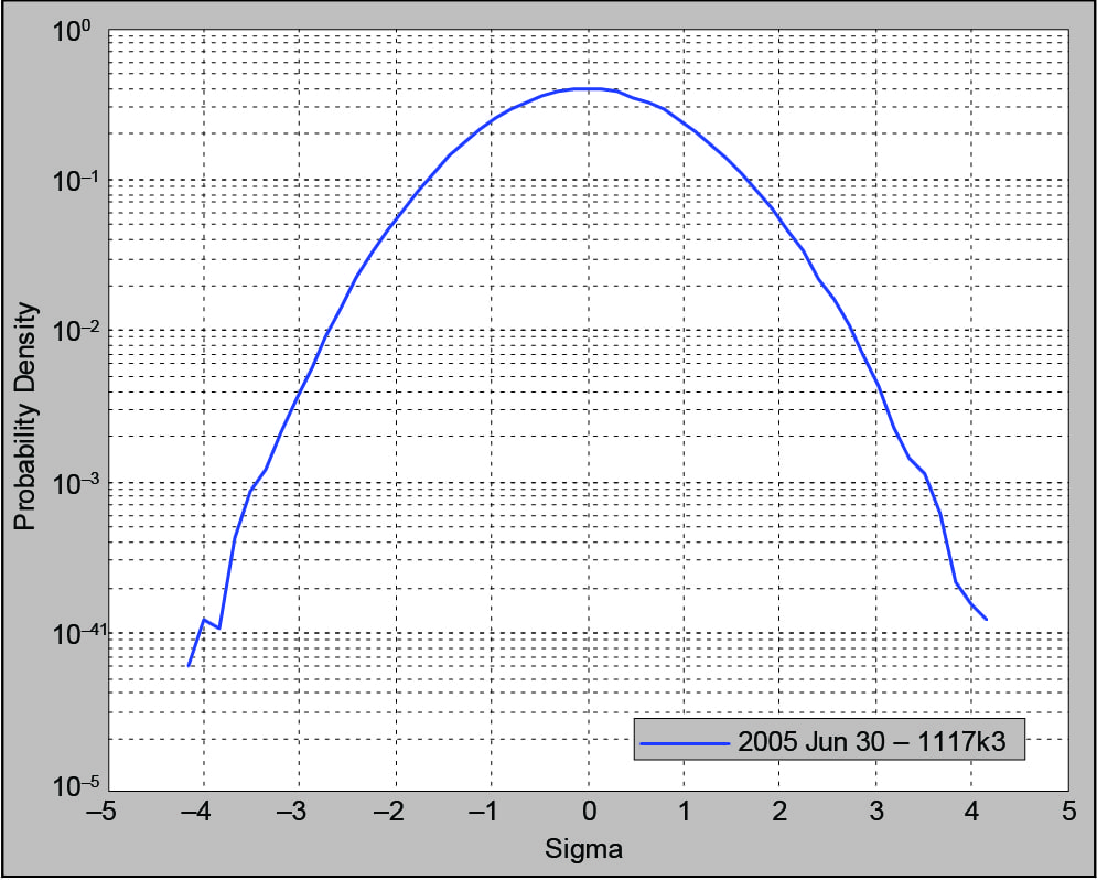
Figure 8. The probability density function for a light bulb test using Gaussian distribution (k = 3).
The PDF in Figure 8 conveys the probability of the signal being at a particular g value at any instant in time. Its vertical units are 1/g, and the area under this curve is exactly 1. Thus, the area under the PDF between any two (horizontal axis) g values is the probability of the measured signal being within that amplitude range. Note that Figure 8 is drawn using a logarithmic vertical axis, which makes the extreme value “tails” more readable.
Various weighted integrals (moments) of this function are determined by the signal’s properties. For example, the first moment is the signal’s mean (μ), the averaged or most probable value. The mean is necessarily equal to zero for a random shaker control signal. The second moment is the signal’s mean square (σ²), and it is equal to the area under the previously discussed PSD. The third moment is the signal’s skew, which indicates a bias towards larger positive or negative values. The skew is always equal to zero for a random control signal. The fourth moment is kurtosis, which measures the high-g content of the signal.
The horizontal axis of an acceleration PDF has units of g peak, not RMS. This axis is often normalized by dividing the g values by the signal’s RMS values. Many signals will exhibit a symmetrical bell-shaped PDF with 68.27% of the curve’s area bounded by ±σ and 99.73% within ±3σ. Such signals are said to be “normal” or Gaussian. A Gaussian signal has a kurtosis of 3, and the probability of its instantaneous amplitude being within ±3σ at any time is nearly 100% (99.73%).
Kurtosis in the Real World
Many “real-life” situations have higher acceleration values than a Gaussian distribution would indicate. Unfortunately, most modern random control techniques assume the control signal is Gaussian with most instantaneous acceleration values within the ±3σ range. This assumption omits the most damaging high-peak accelerations from the test’s simulation of the product’s environment, thereby under-testing results. A Gaussian waveform will instantaneously exceed three times the RMS level only 0.27% of the time.
The situation can be considerably different when measuring field data, where amplitudes exceed three times the RMS level as much as 1.5% of the time. This difference can be significant because it has been reported that most fatigue damage is generated by accelerations in the range of two to four times the RMS level.² Significantly reducing the amount of time spent near these peak values due to using a Gaussian distribution can significantly reduce the fatigue damage caused by the test relative to what the product will experience in the real world. As such, Gaussian distribution is not very realistic.
Present-day methods of random testing may be unrealistic for some simulations because they fail to account for the environment’s most damaging content. Furthermore, random testing with Gaussian distribution will result in a longer time-to-failure because the higher accelerations responsible for failure are omitted. Therefore, Gaussian random testing, for all its advantages over traditional sine testing, has its disadvantages, and a better method of testing products is needed.
Vibration Research developed Kurtosion® to allow engineers to run a random vibration test with a user-specified kurtosis of 3 or greater. Kurtosion uses feedback to force the control signal’s PDF to have broader tails. It includes more intense peak accelerations more often than a Gaussian controller. This method permits the adjustment of the kurtosis level while maintaining the same testing profile and spectrum attributes. With this new technique, a random vibration test is best described by a PSD and an RMS versus time schedule and an additional kurtosis value. Engineers can easily measure the required kurtosis parameter from field data. This process is similar to standard random testing but takes one step closer to the field vibration.
In Figure 8, the data set has a kurtosis value of three (Gaussian distribution) and a smooth distribution with few large amplitude outliers. Figure 9 shows a data set with a kurtosis value of five. The tails extend further from the mean, indicating a large number of outlier data points. Figure 10 shows the contrast between the PDFs of a Gaussian distribution and a higher kurtosis distribution.
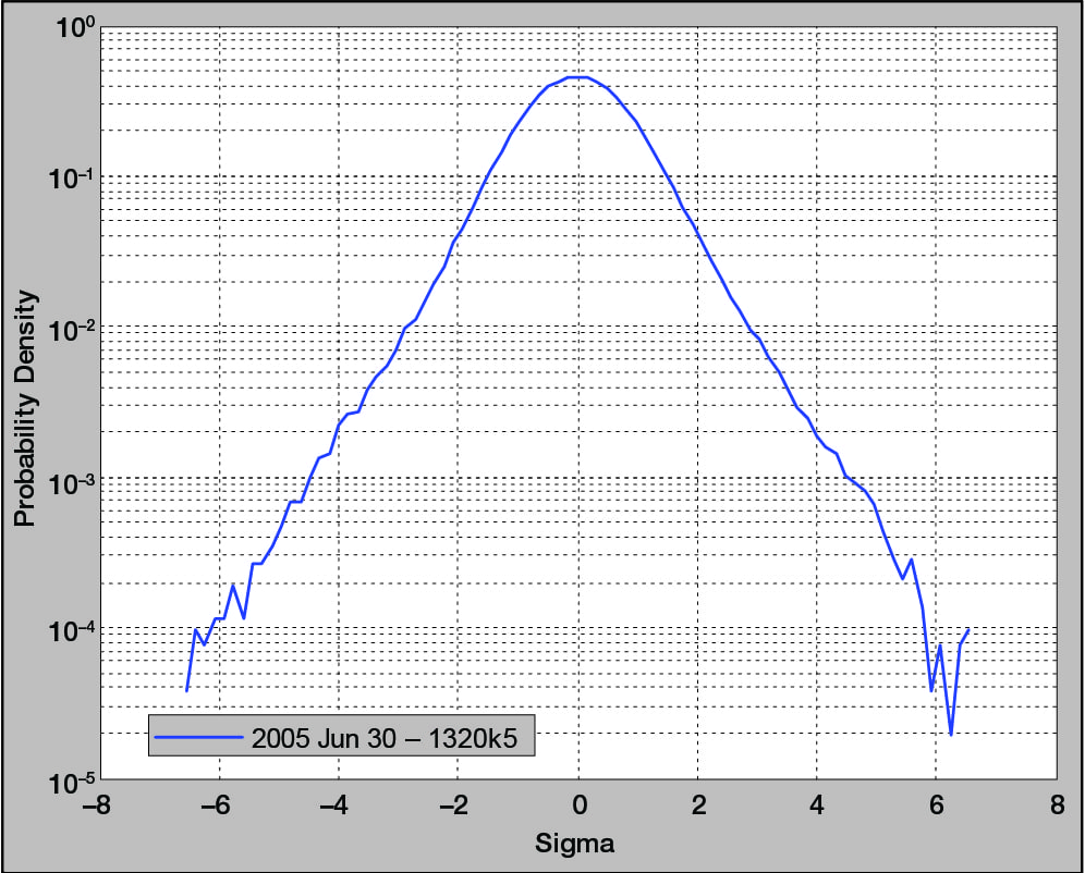
Figure 9. The probability density function for the light bulb test using kurtosis control (k = 5).
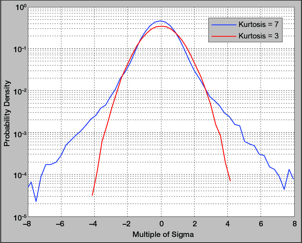
Figure 10. A comparison of kurtosis values 3 and 7. Note how the higher kurtosis value includes higher peak accelerations.
Although the two data sets may have the same mean, standard deviation, and other properties, there is a fundamental difference between a Gaussian and controlled-kurtosis distribution. The Gaussian data set has data points closely centered on the mean, while the controlled-kurtosis distribution has larger tails further from the mean.
Other Testing Options
In modern years, it has become feasible to record a long time-history waveform and then play it back as a shake-test control reference. Vibration Research has pioneered software such as Field Data Replication (FDR) and hardware such as the ObserVR1000, a portable 16-channel data acquisition system. While FDR is the preferred solution for many cases, it is not a replacement for random vibration testing. FDR provides an exact simulation of one instance of the environment. Random provides a statistical average of that environment. Where FDR might exactly capture what one driver experiences while driving a prescribed route, random represents the average of thousands of different drivers trying to follow the same course. While an FDR recording uses massive amounts of memory, a random reference requires very little.
Read: Should I Use a Random or a Field-Data Replication (FDR) Test?
Mixed-mode testing can also produce random signals with high kurtosis, although differently than Kurtosion. Sine-on-random tests can simulate specific environments with random and tonal components, such as an aircraft package shelf experiencing both random air loads and engine harmonics. Random-on-random tests superimpose narrow-band random noise on broadband random noise. These tests are claimed useful to simulate aircraft gunfire reactions. Both test types model a specific class of environment and require a more complex setup.
Conclusions
Overall, random vibration testing is an excellent general-purpose tool for environmental vibration simulation. It is more efficient, precise, and realistic for this purpose than sine testing. Although random vibration testing is not perfect, the testing industry should use the techniques extensively in their screening and qualification procedures.
Last updated: November 27, 2023