Computer-aided design (CAD) is an efficient and accessible alternative to experimental modal testing. Engineers may use modal data from CAD finite element (FE) models for structural design and development.
While these multi-dimensional models are a beneficial tool for visualization, estimation, and analysis, the engineer must select analysis parameters that reflect the observed response as closely as possible. We will discuss several best practices for FE modal analysis, particularly the accuracy of an unconstrained model.
Constraints and Simulation Accuracy
The accuracy of FE modal analysis is largely influenced by the fixture design. A test item can be constrained or unconstrained—that is, it can be attached to one or more mounting points or freestanding. The fixture design may depend on the purpose of the analysis (modal substructuring, estimation of modal parameters, design validation, etc.), although some methods are more accurate overall.
An unconstrained method is a standard approach that can produce favorable results, but engineers must consider the effect of translational and rotational degrees of freedom.
The first six vibrational modes identified in an unconstrained FE model (three translational and three rotational) are associated with the six degrees of freedom at 0Hz. These rigid body modes represent the structure’s movement in the six directions of motion. The engineer must discard this data after recording to ensure an accurate analysis. The resonant frequencies that follow should align with the real-world response.
Vibration Research conducted a study to assess the accuracy of analysis with an unconstrained FE model. The engineer performed an experimental modal analysis with a shaker head expander and followed with an FE analysis of the expander. The frequency analyses were then compared to determine the accuracy of the FE analysis. The following describes the setup of the FE analysis in SolidWorks and compares the results to the experimental data.
Experimental Analysis of a Head Expander
Experimental modal analysis was performed on a 15” head expander for an electrodynamic shaker to determine its resonant frequencies. The engineer used a force-sensing impact hammer to excite the DUT and an accelerometer and the ObserVR1000 hardware to record the data. They performed data analysis with ObserVIEW Modal Testing software.
The engineer designated nine degrees of freedom (DOF) on the expander and suspended the expander by a cord (Figures 1 and 2). They used a roving hammer method, where an accelerometer was mounted at the center of the DUT, and the hammer was moved to each DOF for excitation. The force-sensing hammer was used to strike the head expander three times at each of the nine DOF, and the accelerometer recorded the response. The response was recorded at the z-axis because it was orthogonal to the face of the head expander.
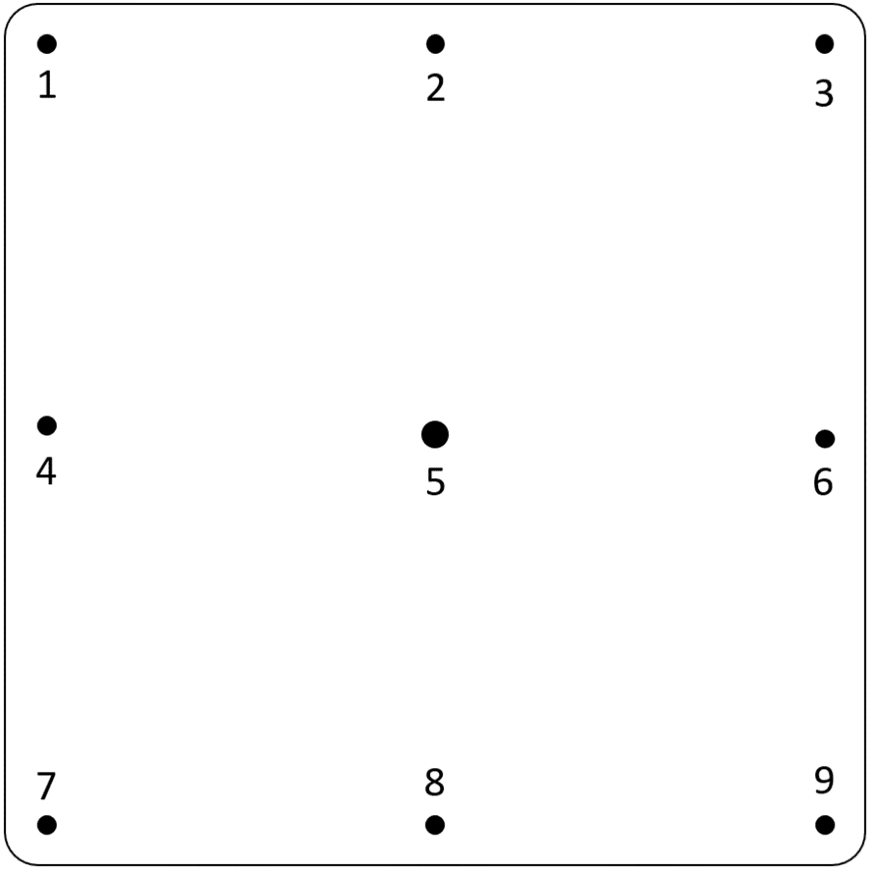
Figure 1. Diagram of the head expander with the designated degrees of freedom.

Figure 2. Head expander suspended by a cord.
A transfer function graph was selected to display the average frequency response of each DOF versus magnitude. The peak frequency values were associated with the primary resonance frequencies ordered by magnitude (Figure 3).
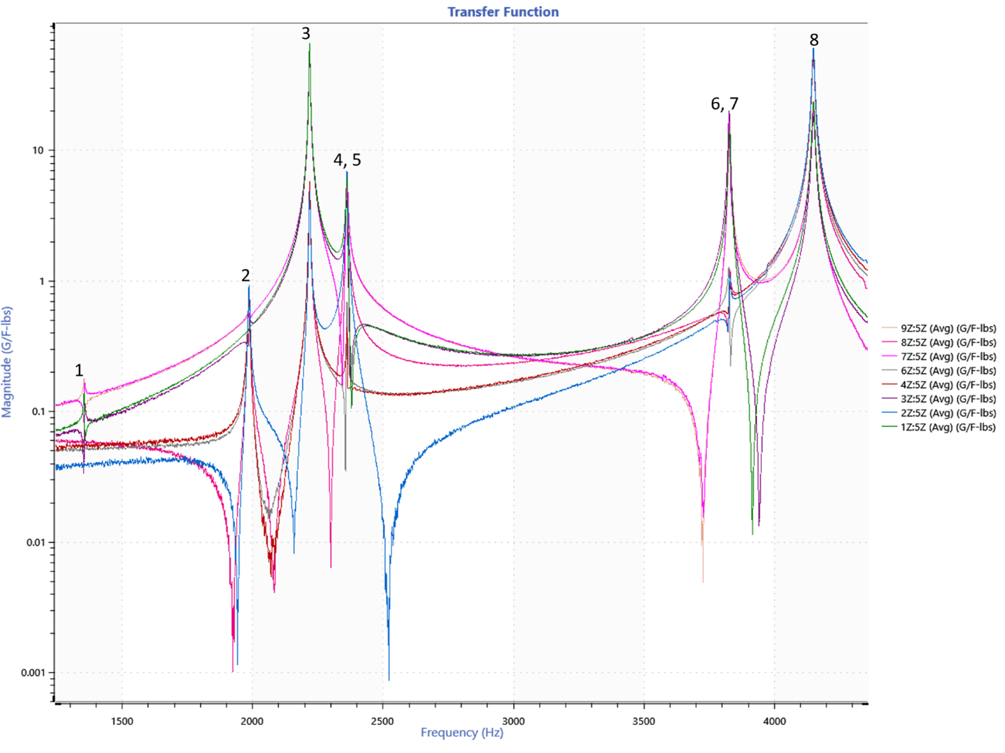
Figure 3. Transfer function displaying head expander frequency response with labeled resonance peaks.
A Nyquist plot was also generated as supplemental information (Figure 4). Each ring of the Nyquist plot corresponds to a resonance.
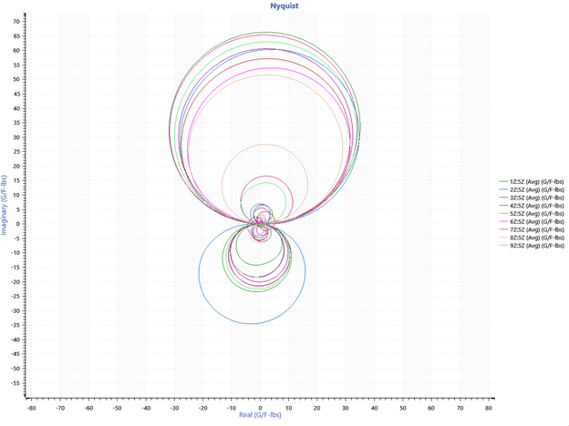
Figure 4. Nyquist plot of experimental data.
SolidWorks Analysis
The engineer generated an FE model of the head expander with the SolidWorks program. They modeled 46 threaded stainless-steel inserts added to the holes of the head expander. Then, they created a simplified hollow cylinder model of the threaded insert with the part’s mass and inserted it into a SolidWorks assembly.
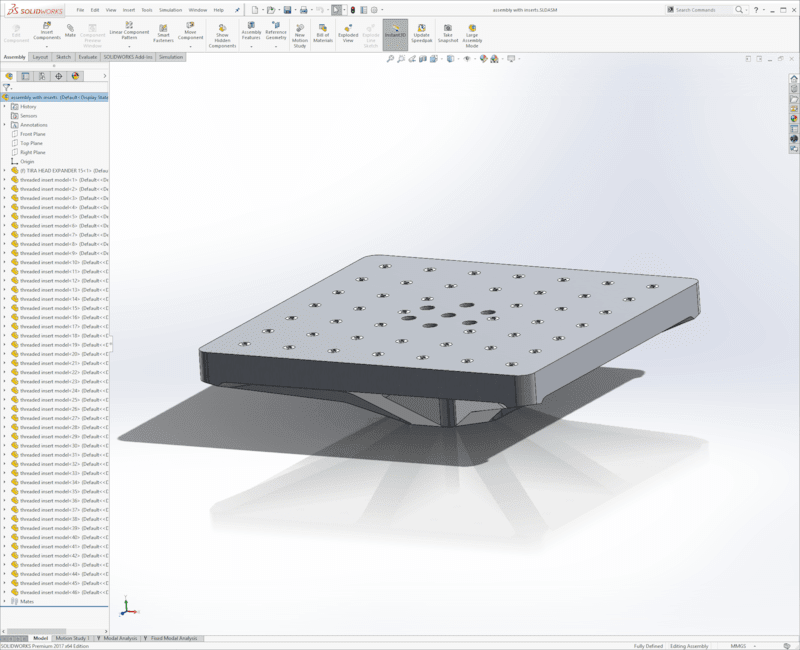
Figure 5. FE model of the head expander created with SolidWorks.
Defining Physical Properties
For greater accuracy, the mass of the model equaled the head expander. The mass was measured with a scale, and then a custom material was made in SolidWorks with a magnesium alloy base template (the head expander is a magnesium alloy.) Finally, the density of the custom material was adjusted so that the total mass of the SolidWorks assembly matched the head expander.
Defining physical properties, such as material and mass, plays an imperative role in the accuracy of the FE model. The material property accounted for the stiffness of the head expander, and the adjustment of mass ensured a proper resonant frequency response.
Unconstrained FE Model
The model was unconstrained to mirror the experimental setup. A frequency analysis of the FE model was performed to identify the resonant frequencies. The operator adjusted the settings in SolidWorks to solve for the first 15 modes to account for the vibrational modes associated with the six degrees of freedom at 0Hz.
As anticipated, SolidWorks identified fourteen vibrational modes due to the unconstrained fixture design. The modes following the three translational and three rotational ones aligned with the first eight peaks on the experimental analysis’s FFT.
How to Properly Perform a SolidWorks (2017) Frequency Study without Fixtures
- Select the New Study dropdown menu > Study Properties.

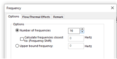
- On the Study Properties dialog box for a frequency study, change the number of frequencies to a value greater than 6.
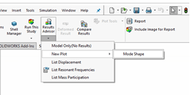
- After the study is complete, view the true mode shapes by selecting the Results Advisor dropdown menu > New Plot > Mode Shape.
- Navigate to the left side of the screen.
- To the right of the tuning fork icon, set the mode shape number to 7 or greater. Seven will be the first true mode shape after the 6 rigid body modes.
- Below the mode shape number, select the Show Colors check box.
- In the upper left corner, select the green checkmark to create a new mode shape plot.
Comparison of Frequency Analyses
The experimental and SolidWorks analyses were compared to determine the accuracy of the FE model (Table 1). The resonant frequencies obtained from both sources were within approximately 3% of one another, and the mode shapes of each resonant frequency aligned.
| Mode No. | Experimental Analysis Freq. (Hz) | Final SolidWorks Model Freq. (Hz) | Model vs Experimental Difference No. (Hz) | Percent Difference |
| 1 | 1354.1 | 1397.5 | 43.5 | 3.21% |
| 2 | 1986.4 | 2046.0 | 59.6 | 3.00% |
| 3 | 2218.5 | 2284.2 | 65.7 | 2.96% |
| 4 | 2361.0 | 2431.1 | 70.1 | 2.97% |
| 5 | 2362.0 | 2432.9 | 70.9 | 3.00% |
| 6 | 3826.8 | 3935.0 | 108.2 | 2.83% |
| 7 | 3829.8 | 3940.2 | 110.4 | 2.88% |
| 8 | 4149.7 | 4281.2 | 131.5 | 3.17% |
Table 1: Experimental and SolidWorks model resonant frequencies of head expander.
Results and Discussion
Each of the modes identified by experimental analysis was displayed on a transfer function graph. A magnitude graph displays the peaks in the frequency response, and an imaginary graph displays the direction of each point on the head expander.
A positive and negative value on the imaginary graph indicates that the resonances are moving in opposite directions. The movement of each point on the FE model corresponds to the directions of the imaginary graph.
Mode 1: 1354 (1398) Hz
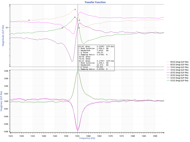
Figure 6. ObserVIEW graph of mode 1. Points 1 and 9 are positive, and points 3 and 7 are negative.
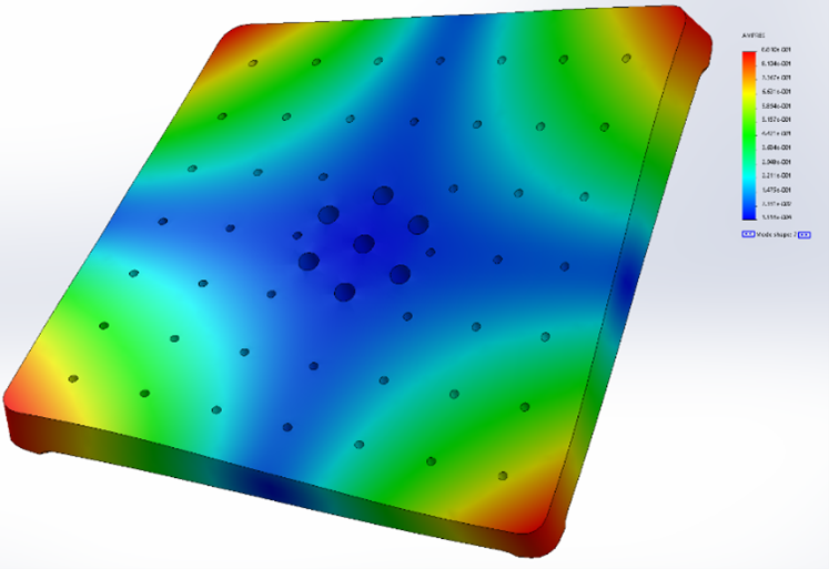
Figure 7. SolidWorks frequency analysis of mode 1 shape.
Mode 2: 1986 (2046) Hz
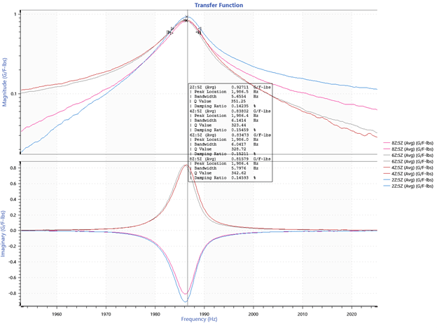
Figure 8. ObserVIEW graph of mode 2. Points 4 and 6 are positive, and points 2 and 8 are negative.
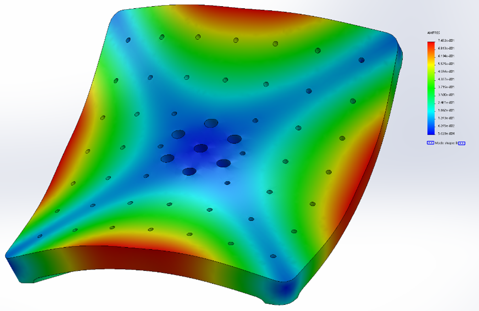
Figure 9. SolidWorks frequency analysis of mode 2 shape.
Mode 3: 2219 (2284) Hz
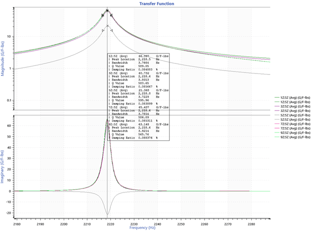
Figure 10. ObserVIEW graph of mode 3. Points 1, 3, 7, and 9 are positive, and point 5 is negative.
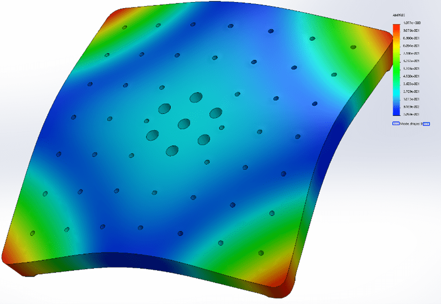
Figure 11. SolidWorks frequency analysis of mode 3 shape.
Modes 4 and 5 are similar in frequency content and mode shape. Mode 5 has the same shape as mode 4 but is rotated 90° CW about the center (Figures 13 and 14).
Modes 4 and 5: 2361 (2431) Hz and 2362 (2433) Hz
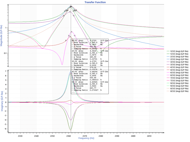
Figure 12. ObserVIEW graph of modes 4 and 5.
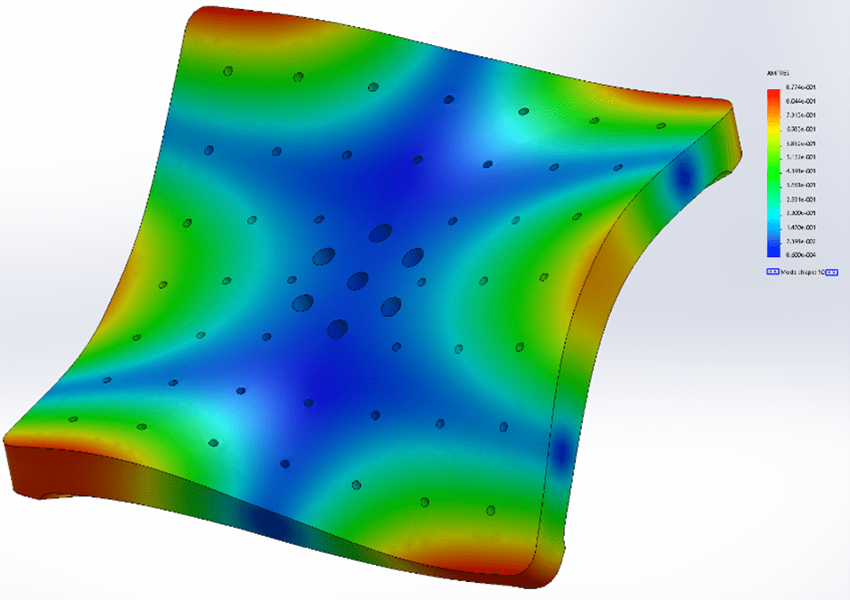
Figure 13. SolidWorks frequency analysis of mode 4 shape.
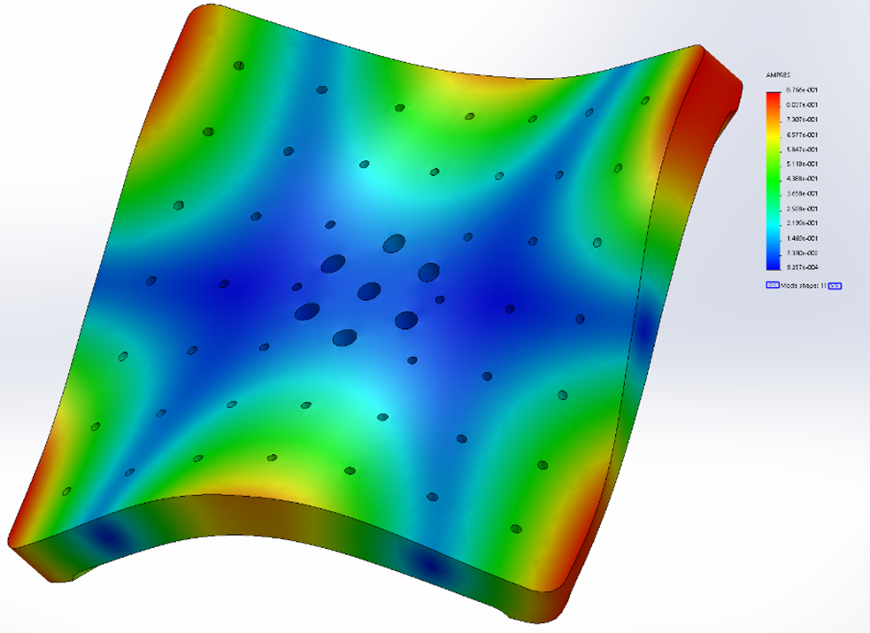
Figure 14. SolidWorks frequency analysis of mode 5 shape.
Modes 6 and 7 have a similar relationship as modes 4 and 5 in that they are similar in frequency content and mode shape. Mode 7 has the same shape as mode 6 but is rotated 90° CW about the center (Figures 16 and 17).
Modes 6 and 7: 3827 (3935) Hz and 3830 (3940) Hz
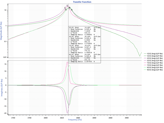
Figure 15. ObserVIEW graph of modes 6 and 7.
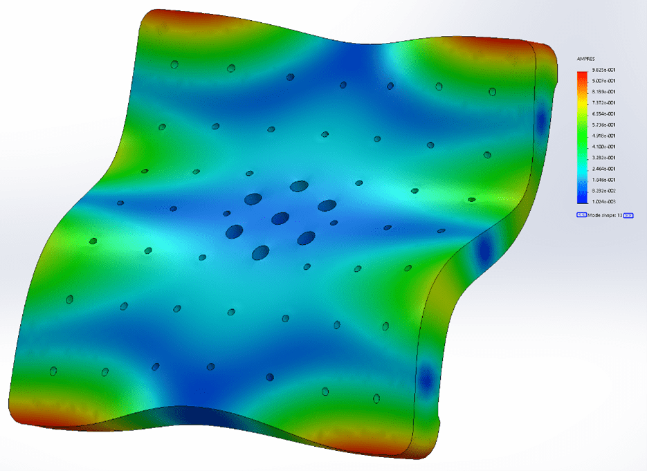
Figure 16. SolidWorks frequency analysis of mode 6 shape.
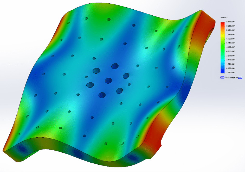
Figure 17. SolidWorks frequency analysis of mode 7 shape.
Mode 8: 4150 (4281) Hz
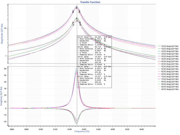
Figure 18. ObserVIEW graph of mode 8. Points 2, 4, 6, and 8 are positive, and points 1, 3, 5, 7, and 9 are negative.
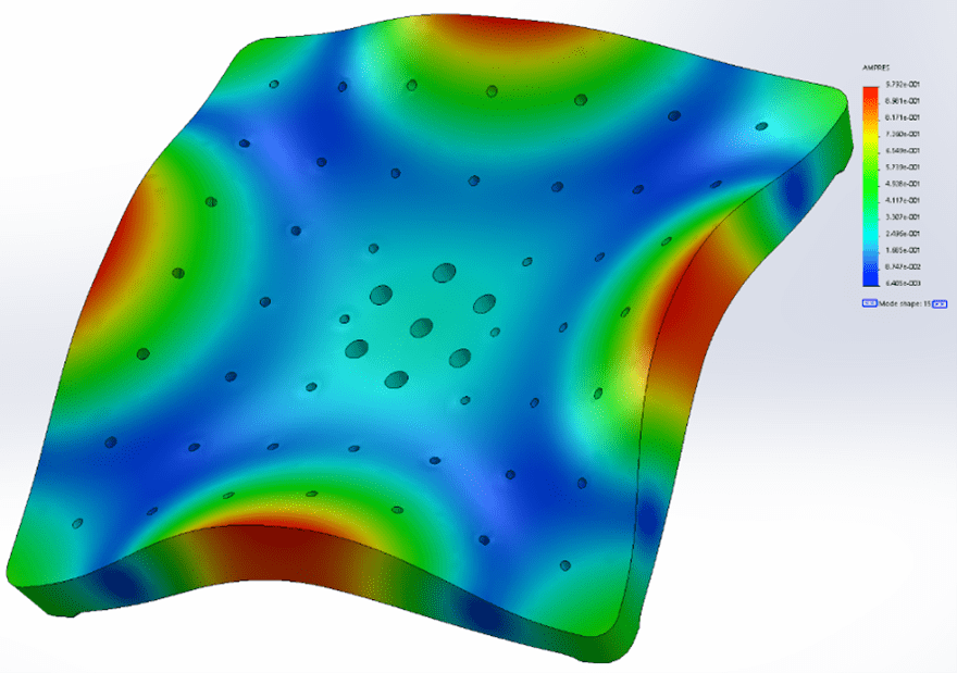
Figure 19. SolidWorks frequency analysis of mode 8 shape.
SolidWorks identified a mode at 3557Hz, but there was no peak in the experimental data. However, there was a node for point 5 at this frequency.
Other SolidWorks Mode: 3557 Hz
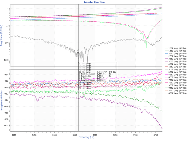
Figure 20. SolidWorks identified mode at 3557Hz.
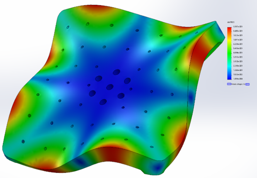
Figure 21. SolidWorks frequency analysis of 3557Hz mode shape.
Conclusion
An FE modal analysis was performed on an unconstrained model to confirm the accuracy of the simulation. The comparison of analyses of experimental data and the FE model displayed a similar frequency and modal response.
The results confirm that an unconstrained FE model produces a frequency response reflective of the observed response, so long as the engineer understands that the first six modes are due to translation and rotation.