Understanding ±3 Sigma Clipping in Random Shake Tests
Random vibration testing presents a host of new and often confusing concepts to the test engineer. Among these, the notion of “clipping” or limiting the excitation signal to ±3 standard deviations has caused undue confusion. This article attempts to explain what 3σ clipping is all about and how it came to haunt us. Given the erosion of written history with time, we will do better at the former objective than the latter.
Generally, we understand that random vibration tests are used to approximate the dynamic stress environment in which components of automobiles, rockets, missiles, and electronic systems “live.” We further understand that such simulations involve shaking components using Gaussian noise, a broadband random signal prone to making structures hiss and roar during excitation.
Gaussian noise describes the random distribution of vibration amplitudes to be statistically normal, or bell-shaped. It implies the theoretical possibility of forced dynamic motion (sensed as displacement, velocity, or acceleration) that includes infinite excursions for a brief instant. While theoretical Gaussian noise considers brief intervals of infinite acceleration, velocity, or displacement, practical testing considers only random motion bound by a crest factor, the ratio of a (finite) peak motion to the root-mean-square (RMS) value of that dynamic signal.
Note that Gaussian amplitude statistics are unaffected by the spectral shape of the random noise.
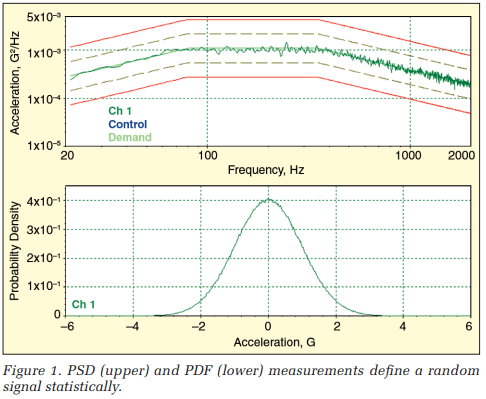
Figure 1 illustrates the graphic description of a typical random signal’s statistical properties. The upper trace in Figure 1 is a power spectral density (PSD) spectrum describing the average frequency content of the signal. The PSD is unaffected by the amplitude distribution of the signal; to the first approximation, it does not care if the profile is Gaussian or not. The lower trace is the probability density function (PDF), which illustrates the Gaussian distribution of instantaneous amplitude. The PDF is unaffected by the frequency content of the signal. Together, these two measurements provide a complete statistical picture of a random signal.
In this discussion of 3σ clipping, we focus on the probability density function (discussed fully in the Appendix). While the power spectral density is an extremely important part of random vibration testing, it is somewhat incidental to this topic. For purposes of this discussion, it is sufficient to recognize the PSD as a plot of (squared) signal amplitude versus frequency and to note that the area under a PSD curve is the signal’s mean square and that the square-root of this area is the signal’s RMS value.
To Clip Or Not To Clip – History, Hearsay, and Heresy
Ask any modern expert in the testing arena why 3σ clipping is used and you are likely to get one of five responses:
- It prevents the shaker amplifier from tripping out on high amplitude peaks, thereby halting the test.
- Clipping minimizes the shaker’s sine force rating required to run a specific random test.
- Limiting extreme Drive peaks minimizes damage to the device under test (DUT).
- Clipping the Drive signal minimizes the required shaker stroke.
- Proper ±3σ clipping makes a squeak-and-rattle test sound “right.”
If you corner a gray-haired guru, you may even elicit an interesting “they got the logic crossed” bit of heresy. In the late ’40s and early ’50s, when the theory of random vibration testing was being evolved and the hardware to implement it was being developed, it was not so easy to make a random noise generator with Gaussian output statistics. A design with enough dynamic range to match the Gaussian distribution out to ±3σ was judged to be a darned good analog signal generator. In other words, ±3σ was considered a minimum requirement or “just good enough.”
Who wrote down the first test or product specification involving ±3σ clipping? Whose thesis first identified limiting the amplitude of a random signal? What problem did he claim this solved? Good questions all; questions that none of a baker’s dozen of well-qualified practitioners queried could answer.
We’ll conduct some experiments that will show Response 1 may hold credence (if your amplifier is of dated design). Explanations 2, 3, and 4 will be shown to be, at best, valid half-truths. Response 5 will be shown to be a matter of poor education. Through it all, the notion of an early minimum requirement being perverted into an accepted modern maximum retains its charm and more than a little credence.
On Clipping and Squeaking
In the “old days,” random waveforms were derived by analog means. Switch selectable nσ clipping was integrated by diode limiting circuits acting on the output of the noise generator. More modern systems used digital noise generation, passing the result through a digital-to-analog converter (DAC) and a subsequent reconstruction or anti-imaging low-pass filter.
Most controller manufacturers chose the least expensive means to implement programmable clipping: the digital signal was restricted in amplitude before it was applied to the DAC. This produced clipping that was less sharp than the earlier analog diode circuits, because the clipping occurred before the reconstruction filter. When Vibration Research first introduced the VR8500 controller, they went to some pain to produce post-reconstruction filter clipping that emulated the superior sharp limiting of earlier equipment. This analog clipping was well accepted for all applications except automotive squeak-and-rattle testing, where some users claimed digital clipping produced quieter results and therefore fewer failed instrument panels.
Vibration Research responded by giving the user a choice of either type of limiting, digital clipping before the reconstruction filter or analog clipping after the filter. Figure 2 illustrates the general arrangement of processing elements of a modern random vibration controller.
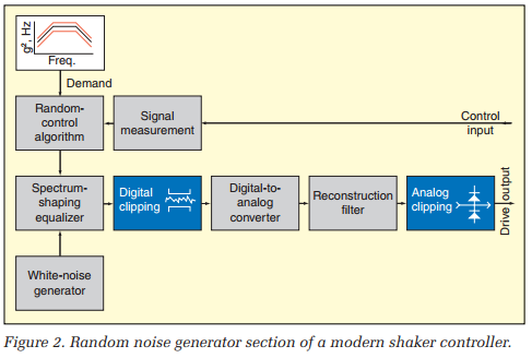
While all manufacturers provide the digital clipping module, the VR 8500 is unique in providing both digital and analog clipping modules. In fact, the 8500 also provides a third clipping option called silent clipping. All three of these were investigated experimentally using the setup of Figure 3.
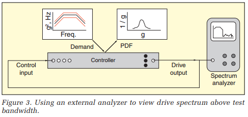
A simple loopback test was conducted using the 20-to-2,000-Hz NAVMAT random profile as the Demand PSD. The test was run at 1 gRMS, and the controller displayed both the PSD and PDF of the Control input signal. Additionally, an external spectrum analyzer was used to audit the Control signal over a broader 20-to-20,000- Hz band.
Figure 4 illustrates the controller’s graphic outputs during a test run made without clipping. The upper trace shows the close match of the Control PSD to the Demand PSD over the 20-to-2,000-Hz test bandwidth. The lower trace presents the PDF of the Control input with a logarithmic vertical axis to emphasize the low-amplitude tails of the PDF. For reference, this trace overlays the theoretical PDF of a Gaussian random variable of 1 gRMS (s = 1). The horizontal axis spans ±6 g that corresponds (in this case) with ±6σ.
Note the close agreement of PDF form between the Control measurement and the Gaussian equation out to better than ±4s. In fact, testing patiently would eventually paint the distribution to ±6s or better. The central portion of the PDF fills in very quickly, but the tails take much longer to populate. As explained in the appendix, it takes 43 times as long to fill the PDF in to ±4σ as it does to paint the central ±3σ. Extending the measured range to ±5σ requires 4,902 times as long, and resolving the function to ±6σ requires a wait of 1,364,435 as long as the ±3σ observation. The important facts in Figure 4 are that the generated signal is clearly Gaussian and that its amplitude span is well beyond ±3σ.
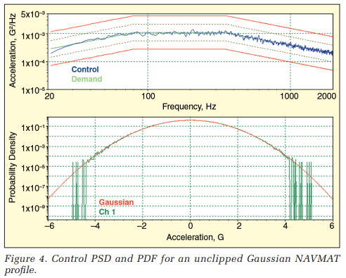
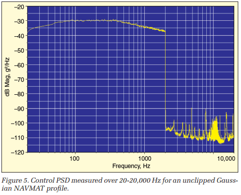
Figure 5 illustrates the audit spectrum of the Control (the Drive) signal measured by an external analyzer running at 10 times the controller’s bandwidth. The left side of this figure (to 2 kHz) duplicates the PSD display of Figure 4. Above 2 kHz, this spectrum shows the out-of-band energy of the Drive is 60 to 85 dB below the Control level. Note the sharp and precipitous drop like a “brick wall” at the upper end of the Control band.
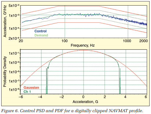
Figure 6 presents the controller’s displays when ±3σ digital clipping is imposed on the NAVMAT profile. Note that the clipping is relatively smooth and gentle, as opposed to a brick-wall transition. In essence, the reconstruction filter has smoothed the amplitude limiting.
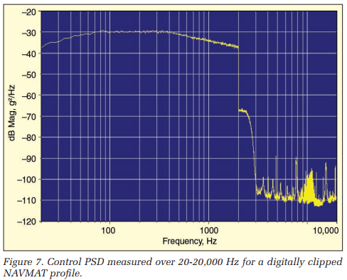
Figure 7 shows the corresponding broadband spectrum. Note that the digital clipping did introduce some harmonic distortion; this is particularly evident in the 2-3 kHz band where we see an increase of up to 40 dB above the unclipped case.
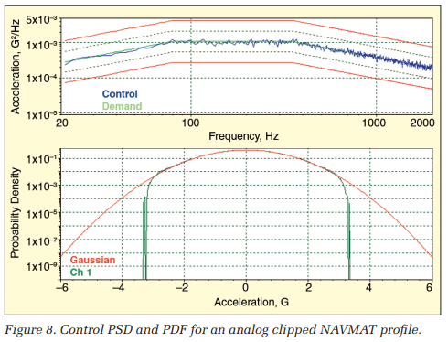
Figure 8 illustrates the application of analog clipping. Note that the ±3σ limits are sharper, reflecting limiting after the reconstruction filter.
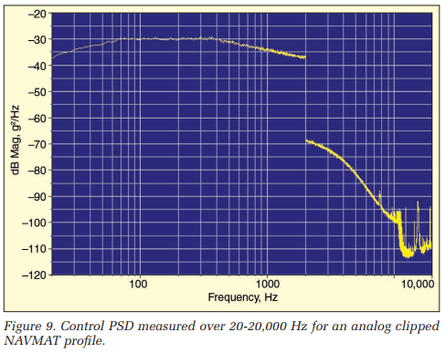
Figure 9 shows the above control band spectrum for the analog clipping case. Note the much-increased energy above 2 kHz extending to more than 10 kHz. This is the reason the analog-clipped signal produced a different sound in some squeak-and-rattle examinations. The added bandwidth of the Drive signal probably excited mechanisms unprovoked by the digitally clipped signal.
Once the physics of the noise difference was understood, Vibration Research set about developing a new clipping technique that would provide the sharp limiting of analog clipping without the associated harmonic distortion. That is, they sought an efficient hard-limiting process that did not introduce high-frequency sound. The resulting procedure is termed silent clipping, and the method of its implementation remains a trade secret.
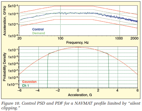
Figure 10 shows the application of ±3σ silent clipping. Note the sharp and definitive limiting in the Drive PDF.
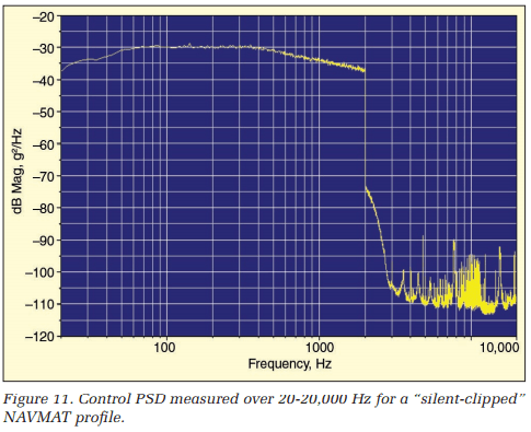
Figure 11 shows the corresponding broadband spectrum. Note that the harmonic distortion is reduced to essentially that associated with soft digital clipping. Therefore, silent clipping embodies the strong points of both analog and digital techniques.
Now it is understood that the sonic difference detected in some squeak-and-rattle tests reflected the presence of high-frequency (out-of-band) content in the Drive signal. As demonstrated by silent clipping, the presence of such added noise has less to do with where you apply a limiting process than it does with the care with which you perform it.
Can You Really Clip the Control Signal?
The preceding experiments were performed on a simple loopback configuration where the Drive and Control signals are identical. What happens when we actually drive a shaker with a clipped Drive? Does the output of the amplifier reflect the limiting? Does an accelerometer sitting on the shaker table detect a clipped Control signal? Clearly, if clipping the Drive does not result in a clipped Control, clipping hypotheses 2, 3, and 4 amount to folklore and wishful thinking.
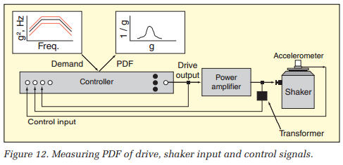
To investigate this important issue, a VR8500 controller, a Haffler Pro 1200 amplifier, an LDS V-203 shaker, a PCB model 288M05 sensor, and an instrumentation transformer were configured as shown in Figure 12. The same NAVMAT profile and 1-gRMS level employed in the previous test were used.
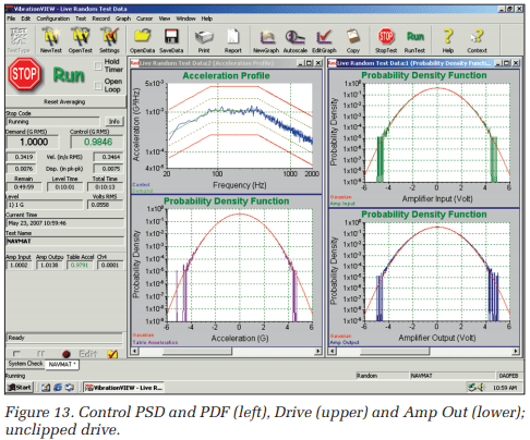
Figure 13 shows the results of an unclipped run of 10 minutes. The left pane shows the PSD and PDF of the Control acceleration. The right pane presents the PDF of the Drive signal (amplifier input) above the PDF of the amplifier’s output (sensed through an instrument transformer). The mV/Volt scale factors for these two signals were chosen so that they too would present with an RMS value of 1. All PDFs were formatted to display a ±6σ horizontal range. Note that all three PDFs (amplifier input, amplifier output, and table acceleration) are exhibiting Gaussian behavior out to better than ±4σ.
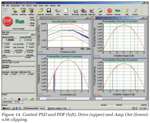
The same test is repeated (for the same duration) in Figure 14 with ±3σ silent clipping applied. Recall from Figure 2 that clipping is always applied to the Drive signal (the amplifier’s input). As the right panel of Figure 14 illustrates, the amplifier’s input is sharply limited to ±3σ. Note that the amplifier’s output also reflects this limiting. However, the clipped voltage applied to the shaker does not result in a limited Control signal. The lower left pane clearly shows the table acceleration experiencing ±4σ, essentially the same range as without Drive clipping.
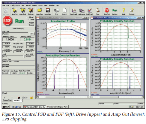
To drive this point home, the test was rerun with more severe clipping. A ±2σ silent clipping level was used in Figure 15. Again the amplifier’s output reflected the clipping level applied to its input, but the Control acceleration experienced a much broader range of amplitudes. Without question, clipping the Drive does not assure the Control signal is limited to a known s level. So it is most unlikely that clipping will limit shaker stroke or force required or do anything to protect your delicate DUT.
Each of the three preceding tests was recorded using RecorderVIEW. The data were played into a MATLAB® program that integrated and double-integrated the measured Control time-waveform and computed PDFs for the acceleration (black), velocity (blue), and displacement (red). The results are presented in Figure 16.
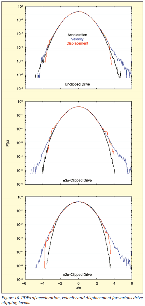
Figure 16 presents PDFs from 10 minutes of recorded data from the unclipped, ±3σ-clipped and ±2σ-clipped tests. The (3.3 million sample) Control signal was integrated twice, using a time-domain trapezoidal approximation. Prior to each integration, the data were passed through a 1-Hz Butterworth high-pass filter to eliminate any DC bias. Normalized (x/s) PDFs with a resolution of 0.05σ were computed for all signals and plotted over a ±6σ span.
While there are slight variations in PDF span between the three tests, it is clear that limiting the Drive signal did not produce an equivalent limit of the Control acceleration or its time integrals. Note that all nine PDFs of Figure 16 exhibit a span of about ±4σ, regardless of the limiting applied to the Drive.
One More Test – Just Some Simulation and Stimulation
Since the results of our shaker experiment suggested limiting or clipping of the Drive signal might not actually restrict the motion requirements of the electrodynamic shaker employed, a second experiment was conducted to verify this finding. In this investigation, we sought to determine if Drive limiting actually impacted shaker stroke requirements. A cautious analyst is always suspicious of open-loop integration, no matter how carefully it is implemented.
Therefore, we sought a simultaneous test measurement of shaker table acceleration and displacement. The former is easy, the latter difficult. We took a novel approach, calling upon analog simulation. The NAVMAT test profile was applied to a well-understood analog circuit representing the V-203 electrodynamic shaker previously discussed. The circuit of Figures 17 and 18 models the small shaker used in the experiments of Figures 12 through 16.
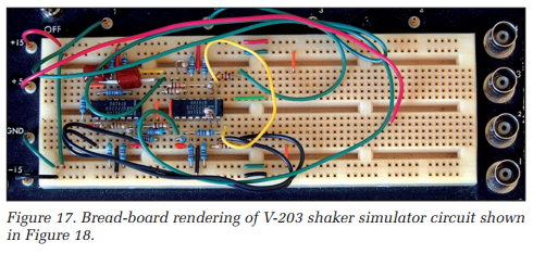
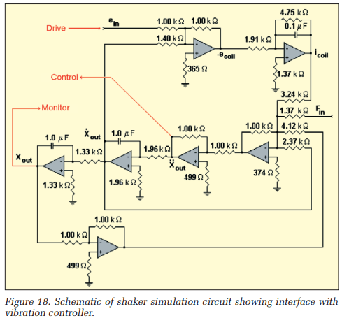
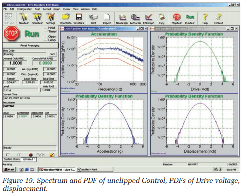
The NAVMAT profile was applied to the simulation circuit of Figures 17 and 18. Two runs were made, the first with no clipping and the second with ±3σ (silent algorithm) limiting of the Drive signal. Figure 19 illustrates the unclipped case; the Drive and the resulting (acceleration) Control and its (double-integral) displacement all exhibit considerably greater than ±4σ signal span.
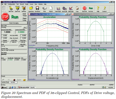
In Figure 20, the Drive signal has been deliberately limited to ±3σ, using the highly efficient Vibration Research silent clipping method. While the Drive voltage applied to the amplifier is clearly limited to this range, the resulting acceleration and displacement signals still have greater than ±4σ, exhibiting their independence from Drive limiting. In fact, whenever the control-loop transfer function is more complicated than a zero-phase, flat-line, clipping of the Drive input, it will have no direct limiting effect on the measured Control signal.
Conclusions, Infusions, Illusions, and Delusions
For many years, ±3σ clipping has been viewed as a defense mechanism by those seeking to protect an item they must test, by those hoping to get a little more performance out of their existing shaker and by those sales types hoping to match a smaller and cheaper shaker to an application. It is likely that all of them have experienced a false sense of security. The truth is that clipping the Drive does not assure any significant change in a shaker’s motion statistics.
It is certainly possible that older shaker amplifiers have been caused to function at higher RMS levels without tripping by clipping the Drive signal. It is also highly probable that amplifiers sensitive to this problem are truly obsolete equipment deserving of replacement by modern solid-state designs with protective input clamping circuits.
Controller manufacturers do not write testing specifications and protocols. If they did, ±3σ clipping would quickly be eliminated from the testing vocabulary as “an old idea that simply did not pan out.” In fact, the pendulum is swinging toward Demand profiles that have accentuated PDF tails for more life-like damage detection. The Vibration Research Kurtosion® algorithm leads the industry in producing Control signals with higher than Gaussian kurtosis. High kurtosis test signals are the antithesis of clipped-signal tests; they provide a higher percentage of high sigma test time and they work as expected!
Almost Everything You May Want to Know About PDFs
A probability density function (PDF) is a type of amplitude histogram drawn with specific scaling. The horizontal axis has the units of the measured variable (g, volt, inch, etc.) This axis normally spans positive and negative values, representing the entire range of the possible instantaneous values the signal may attain.
The area under the PDF curve is always unity (and non-dimensional). Therefore, the units of the vertical axis are the reciprocal of the horizontal axis units. This scaling differentiates a PDF from a raw histogram from which it is normally computed. A raw histogram has counts or occurrences as its vertical axis units. In fact, measuring a histogram is a counting process.
A PDF is really a mathematic abstract. Like a Fourier transform, it is a continuous function of amplitude. and the horizontal axis may span ±∞. As with other sophisticated signal statistics, it is implemented as a discretized function of sampled data. That is, a stream or time history of sampled digital amplitude values is used to compute PDF values at a finite number of points spanning the ± full-scale of the measurement system.
Each (of n) horizontal PDF locations represent a small span of amplitudes, just as each point in an FFT spectrum represents the output of a narrow-band filter of resolution bandwidth. The points are equally spaced in amplitude so that the horizontal axis has resolution and spacing of ΔX = 2·Xfull-scale/n. A bank of counters implements the measurement; these are all cleared to zero count prior to measurement. Each time an ADC sample is measured, its amplitude is used to address one (of the n) counters, whose ΔX encompasses the sample’s amplitude. This single counter is incremented, and attention shifts to the next signal sample. All counting is halted to end the measurement. The PDF amplitude for the ith point is computed as the counts in the ith counter divided by the total of all counts in all counters and by ΔX.
Having a unit area under the PDF curve, p(x), is of fundamental importance. A properly scaled PDF allows evaluating the probability that the signal’s instantaneous amplitude is between Xa and Xb. This is simply the area under the PDF curve between x=Xa and x=Xb. That is:

and therefore:

The PDF, p(x), also exhibits two important properties that link it to statistical functions in the time and frequency domains. In particular, the signal’s mean value μ and its variance, σ2, can be evaluated from the (first and second moment) integrals:

and:

Note that the square root of the variance σ is called the signal’s standard deviation. These same statistical parameters can be extracted from a time-history, x(t), by integration in time. Specifically:


Note that the signal mean-square defined by Equation 6 is identical to the area under a PSD curve. The RMS value may be seen to be equal to √(μ2 + σ2). Whenever a dynamic signal has a zero-valued DC component, μ is zero and the RMS is identical to the standard deviation, σ. This is always the case with random signals used for shaker testing.

It is interesting to note that when you auto correlate x(t) in accordance with Equation 7, the amplitude at lag time t=0 is equal to σ2 + μ2. As the lag time approaches infinity, the correlation amplitude collapses to μ2. That is, the autocorrelation amplitude varies between the mean square and the square of the mean. It is reassuring to find that all of the traditional signal-statistic functions computed in time, frequency or amplitude domains recover the signal mean μ and standard deviation σ.
The first and second-order moments of the PDF identify the mean and variance of a signal. Higher-order moments of the PDF provide additional statistics exclusive to the amplitude domain. Two of the most important of these are skew and kurtosis, the third and fourth-order moments defined by Equations 8 and 9, respectively. Skew describes the symmetry of the PDF, while kurtosis describes the spread of the tails.


Is This Normal?
PDFs can exhibit many different shapes, reflecting various signal characteristics. For example, a square wave’s PDF has two sharp spikes at the ±peak values and is zero everywhere else. A triangle wave has a uniform height PDF over the span between its ±peak values and is zero outside of this range. A sine wave of peak amplitude α has a PDF defined by the equation:
![]()
Different types of random signals can also exhibit various PDF forms. However, a broad range of natural phenomena, including vibration, exhibit the familiar bell-shaped PDF we have come to know as a normal distribution. Many normal PDFs are modeled well by the classical Gaussian distribution:

Figure 21 plots the theoretical distribution of Equation 10. Note the strong similarity of the measured PDF shown in Figure 1. In Figure 21, the area under the ±1σ span from the mean is marked in blue. The signal amplitude is within this range 68.3% of the time. Clearly, the signal’s amplitude spends very little time (less than 0.27%!) outside of the ±3σ span. From this plot you can see the origin of the old vibration test engineer’s saw, “3σ is a reasonable approximation of infinity.”
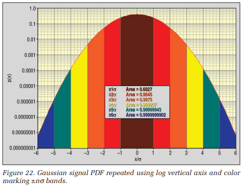
Figure 22 reinforces this notion. Here the vertical axis is changed to a logarithmic axis, displaying a much broader range of probabilities and affording us a better view of the tails that describe the high-amplitude, low-probability events. The color-coded areas illustrate that the signal spends 68.3% of its time within ±1σ, 95.5% within ±2σ, 99.7% within ±3σ, and 99.999937% within ±4σ. In short, it paints a clearer picture of the infrequent extreme events. We used this view in evaluating the experiments here.
A Gaussian distribution exhibits a skew of μ(3σ2+μ2) and kurtosis of 3σ4+6σ2μ2+μ4. Those Gaussian signals used to drive shakers have a zero DC value (μ=0). So their skew is zero and their kurtosis is 3σ4, which is commonly expressed by a normalized kurtosis value of 3.
The tables of the Gaussian distribution are normally presented in normalized form. That is, the tables present p(x) values and areas under the p(x) curve for distribution with zero mean and unit variance. In fact, any data set can be normalized by the use of a simple transformation:
The required mean μx and standard deviation σx can be evaluated using Equations 5 and 6. The PDF of the z, p(z), has the following properties:
- μz=0
- σz2=1
- Skewz=0
- kurtosisz = 3
What Time Did Gauss Have In Mind?
We recognize that area under the PDF represents non-dimensional probability. That is, the area bounded by the curve and two vertical lines define the fraction of time that the signal will be between the amplitudes represented by the lines. In running the experiments discussed herein, we note that the PDF display “paints in” from the center out, as intuition would suggest. That is, the central, most probable, amplitudes are encountered immediately while the less probable high-σ amplitudes occur much less frequently.
All of this is satisfying, but raises a basic question: How long must I wait for an event bounded by ±nσ to occur? The answer is that this depends on the bandwidth of the Gaussian random signal being generated.
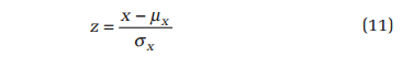
An experiment’s measured PDF is computed from samples taken from a time-history. Let’s re-express the information on the PDF based on that understanding. As a starting point, consider the 0.6827 probability area bounded by ±σ. This suggests that better than two out of three amplitude samples will fall within one standard deviation of the mean, or about one in three will exceed the ±1σ range. In like manner, about one in 22 samples will exceed ±2σ, while about one of every 370 samples will exceed ±3σ and one in 15,780 will exceed ±4σ. This relationship is plotted in Figure 23. It amounts to an alternative-format graph of the CDF, the integral of the PDF.
Figure 23 is deliberately plotted with the number of samples required as the x-axis variable. This allows scaling of the independent variable as time, by multiplying the x-axis values by a reference time separating statistically independent time samples.
When a vibration controller measures the PDF, the sample rate is determined by spectral considerations. The samples are not statistically independent of one another; they are highly over-sampled or redundant. We can estimate the time between statistically independent samples from the 3 dB bandwidth of the PSD describing the Control signal. As shown in Figure 2, a vibration controller forms the Drive signal by shaping the spectral amplitude of a white noise signal. The shaping transfer function is determined by the Demand profile and the dynamics of the amplifier/shaker/DUT being excited. In a simple loop-back test, the Drive and Control signals are identical and the shape of the demand profile defines the 3-dB bandwidth of the shaping filter. The PSD for a NAVMAT profile is shown.
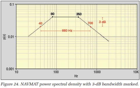
The PSD for a NAVMAT profile is shown in Figure 24. This signal is flat from 80 to 350 Hz. Outside of this span, it falls off at 3 dB/ octave. Therefore, the signal is –3 dB below the central plateau at 40 and 700 Hz, defining a –3 dB bandwidth, Δf–3dB, of 660 Hz for the shaping filter.
The rise time τ of a system (such as a filter) is defined as the time it takes the output signal to swing from 10% of full-scale to 90% of full-scale in response to a stimulating step input. This characteristic reflects the system’s transfer function. The rise time is well estimated by the relationship:

In the case of the NAVMAT signal, the rise time is:

For the VR8500 controller, the full scale is 10 volts. In all of the loopback tests, a scale factor of 1000 mV/g was employed. Therefore, the full-scale acceleration is 10 gpeak. This means, when a 1 gRMS random signal is generated, the full scale corresponds to 10σ. So a 10% to 90% full-scale swing corresponds to changing by 8σ in 530 μsec or 1σ in 66.3 μsec.
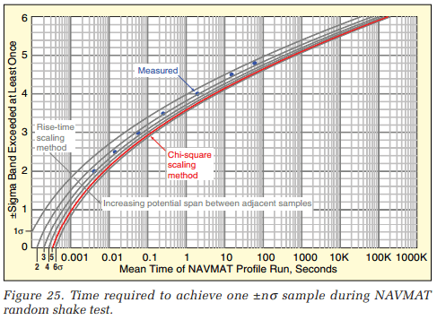
Figure 25 presents a family of curves reflecting the rise-time scaling method. Each of these was derived by multiplying the horizontal statistically independent sample axis of Figure 23 by a multiple of 66.3 μS. Thus, the traces reflect a maximum change between adjacent samples of 1σ, 2σ, 3σ, 4σ, 5σ, and 6σ. In Figure 25, this scaling estimate is compared with two other means of evaluating the time required to acquire a single sample exceeding ±nσ.
The red trace in Figure 25 reflects evaluating a time-scale factor by a very different means. This evaluation technique is termed the chi-square scaling method. It requires measuring the mean and standard deviation of the square of the random signal. These measurements were performed upon a recorded Drive signal using RecorderVIEW and MATLAB. The resulting 340 μsec scale factor agrees very closely with the rise-time scaling line for adjacent points separated by 5σ or less.
The chi-square method depends upon the basic property of a Gaussian random signal. Specifically, it depends on the fact that the variance of a Gaussian signal is chi-square distributed. That means that if the amplitude of each signal sample is squared, the PDF of the squared signal will exhibit a chi-square shape as shown in Figure 26. Note that the shape of this probability density function is defined by three variables: the mean, the standard deviation, and the number of degrees of freedom (DOF).
A DOF is simply a statistically independent sample. For a single DOF, the chi-squared PDF is exponential in shape. As the number of DOF increases, the chi-square distribution begins to develop a peak near its mean value.
The chi-square distribution has two important characteristics for this application. The mean value μchi 2 is proportional to the number of DOFs, while the standard deviation σchi 2 is proportional to the square root of twice the number of DOF. The mean and the variance σ2chi 2 of the squared random sequence can be evaluated from Equations 5 and 6. Knowing these two parameters allows the number of DOF to be calculated as:

Therefore, a scale factor is derived by averaging the mean and variance of a block of N samples of the squared Gaussian noise measured at equally spaced time intervals, Δt. The DOF of this block (DOF≤N) is computed using Equation 14. The (seconds/ sample) scale factor SF is evaluated as:
(1) 
Finally, MATLAB and RecorderVIEW were used to actually measure the mean time required to exceed various sigma levels. Well-separated disparate blocks of the sampled random waveform were extracted from a long recording. For each block, the number of samples exceeding a given sigma level was recorded. The results from a large number of blocks were averaged. The time length of a block (N·Δt) divided by the averaged number of sigma-exceeding samples is presented in Figure 25 as blue circles.
Authors: George Fox Lang, Independent Consultant, Hatfield Pennsylvania & Philip Van Baren, VP/Engineering, Vibration Research
Published: Sound & Vibration magazine, March 2009 pp 9-16.
Appeared in: Sound & Vibration Magazine, March 2009 pp 9-16.3.
Random vibration testing presents a host of new and often confusing concepts to the test engineer. Among these, the notion of ‘clipping’ or ‘limiting’ the excitation signal to “±3 Standard Deviations” has caused undue confusion. This paper attempts to explain what 3 σ clipping is all about and how it came to haunt us. Given the erosion of written history with time, we will do better at the former objective than the latter.