Introduction
It has long been known that excessive vibration breaks things. Classic cases of failing bridges [e.g. Tacoma Narrows Bridge (1940)] and rocket boosters [e.g. Titan Rocket (1959)] can be seen in videos on the web. This tutorial focuses on the failure of products subjected to a vibration environment, that is, they are mounted on a vibrating base. One question facing everyone from the designers to the purchasers of such a product is, “How much vibration will cause failure?” A related question is, “How long will the product last in a specified vibration environment?” This tutorial presents three test methods that can be used to answer these questions.
1. Direct Vibration Environment Simulation Test Method
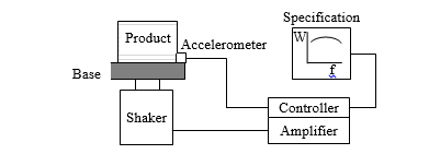
Figure 1. Direct Vibration Environment Simulation Test
A test using the direct vibration environment simulation method is illustrated in Fig. 1. The product is mounted on a vibration shaker using a base fixture that simulates the real-life situation. At least one accelerometer is used to measure the base vibration level. The base vibration environment can be sinusoidal, periodic, random, or some combination. Random vibration is often specified by a power spectral density (PSD) of acceleration, denoted by W(f) which gives the mean-square amplitude of the acceleration per frequency bandwidth in units of g2/Hz [or (m/s2)/Hz, or (in/sec2)/Hz] over a range of frequencies.
If the vibration environment is specified, then a signal controller for the shaker input must be used. The system consisting of the input electronics, the shaker, and the base fixture will not have a flat frequency response, so the controller modifies the shaker input signal to obtain the specified vibration levels as measured by the base accelerometer(s). This is illustrated in Fig. 2.
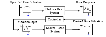
Figure 2. Controller Used to Obtain Specified Base Vibration Level
There are two limitations to this method. One is the time duration of the test must be the length of time given in the specification and this may be too long for practical product testing. Therefore, a method for time compression or accelerated testing may be needed. It is not sufficient to double the vibration amplitude and assume the failure will occur in half the time. This is addressed in the second test method below.
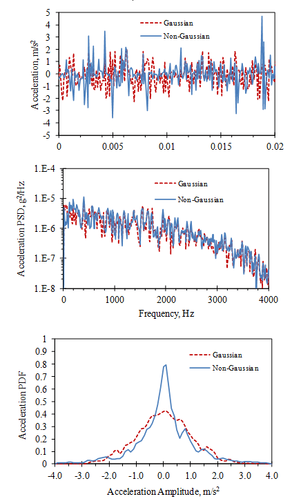
Figure 3. Example of Gaussian and Non-Gaussian Signals with the Same PSD
A second limitation occurs when the vibration environment is specified using a PSD, as in the case of random vibration. It is often assumed that the amplitude of a random signal has a Gaussian (normal) distribution over time in which case the PSD specification is sufficient. However, Fig. 3 illustrates two signals with the same PSD and RMS (root-mean-square) levels but with different amplitude distributions, given by their probability density function, PDF. In this case, the non-Gaussian signal has higher peaks and can cause more rapid failure. This is addressed in the third test method below.
2. Accelerated Test Method Using the Cyclic Fatigue Power Law
The common experience of breaking a paper clip illustrates that the questions in the introduction of “how much?” and “how long?” are related to each other. If a paper clip is bent open to 90° it usually doesn’t break. If it is bent back to flat and then repeatedly bent to 90° and back several times, it eventually breaks. Now, if the same process is repeated with a similar paper clip but only bent to 45° each time, it usually takes more cycles of bending and flattening to break it. This is an example of cyclic fatigue which was first studied in the mid-1800s relating to the sudden fracture of railroad car axles. Axles that were clearly strong enough to carry the carload would sometimes break after extended use.
This could not be explained using the accepted view of the strength of materials. Hooke (1678) had observed that most objects act like a linear spring: its deflection is proportional to the force applied. Applying this to the quantity of stress, s (force per unit area), Hooke’s law is stated as where ε is the strain (stretching per unit length) of the object and E is the elastic modulus (stiffness) of the object’s material. For small strains (typically less than 0.1 %) this linear relationship holds true for many materials. However, for larger strains the stress-strain relationship is non-linear. Fig. 4 shows a typical stress-strain curve for AISI 4340 steel from a tensile test.
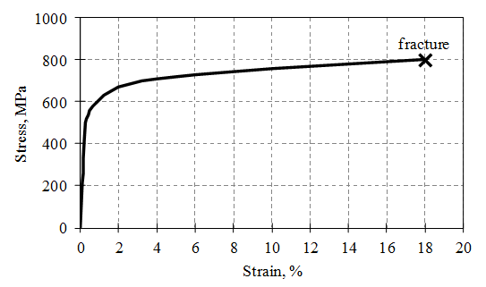
Figure 4. Stress-Strain Curve for AISI 4340 Steel
Up to stress of about 500 MPa, the curve is linear (e.g. twice the stress causes twice the strain). The slope gives the elastic modulus, E = 210,000 MPa, for the material. In this range the deformation is elastic (reversible) and, historically, it was generally assumed there was no permanent damage to the material. Above stress of about 500 MPa (called the yield strength), the curve is non-linear and much of the deformation is plastic (permanent and not reversible). At about 800 MPa (called the ultimate tensile strength) the material fractures under the static load.
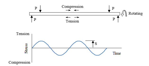
Figure 5. Sinusoidal Stress Loading for Basic Cyclic Fatigue Tests
Wohler (1870) performed laboratory tests with a number of rotating railroad axles under different levels of bending load and measured the number of cycles required to cause failure. A static bending load, P, on a rotating axle causes cycling of the stress from tension to compression at any particular point on the axle as shown in Fig. 5.
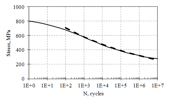
Figure 6. Example of the S-N graph for AISI 4340 Steel
Wohler created the “S-N” graph (Fig. 6) to present these results. The maximum applied stress, S, is plotted vs. N, the number of cycles causing the failure, on a log scale.
Comparing Figs. 4 and 6, it can be seen that cyclical stresses above the yield stress (causing plastic deformation) result in failure before 103 cycles. This is called low cycle fatigue (LCF) and is highly non-linear and difficult to model. This tutorial focuses on the other case, where cyclical stresses below the yield stress (causing elastic deformation) result in failure after 103 cycles. This is called high cycle fatigue (HCF) and is suitable for linear models.
Over many years a large amount of S-N data has been collected for a variety of materials including the influence of a number of design variables, such as surface finish, notches, and fillets, heat treatments, etc. The general consensus as to the cause of failure in the HCF range of stress is explained by the theory of fracture mechanics. Microscopic defects in the material’s molecular structure grow as the stress is cycled even though this is not evident to the eye. Eventually, the defects grow into cracks and the material breaks. [e.g. Paris, et al. (1961)]
Several modifications have been made to the S-N curve to account for different loading conditions found in many situations. Goodman (1899) and others considered cases where the mean value of the loading is not zero. Since vibration excitation is generally assumed to have a mean value of zero, these cases are not considered here.
The S-N curve (Fig. 6) clearly shows an inverse relationship between the maximum applied stress and the number of cycles to failure. Basquin (1910) proposed using an exponential power law equation to fit the HCF range of the S-N data of the form where c and b are constants. Typically the constants b and c are determined using the failure stresses at N = 103 and 106, denoted by SE3 and SE6, respectively. Solving for b and c using Eq. (2) at these two points (with S given in MPa) gives
Using the example in Fig. 6, SE3 = 580 MPa, SE6 = 320 MPa, b = -0.086, c = 1050 MPa. This result is shown as a dashed line on Fig. 6.
If a product is being excited sinusoidally at a frequency fo (cycles/sec), where the maximum stress occurring is S, then the time to failure, tf, is predicted to be: Unfortunately, the uncertainty in predicting the absolute time to failure is largely due to the slope of the S-N curve. Using Fig. 6, peak stress of 400 MPa predicts failure at 100,000 cycles. However, a 50% increase in stress to 600 MPa (which could easily occur at a stress concentration such as a bolt hole) predicts failure at 1000 cycles. Therefore, Eq. (4) is more frequently used to predict a relative scaling in the time to failure for different stress levels. The most widely used accelerated test method uses the slope of the S-N curve (Fig. 6) to properly scale the time duration and amplitude of the vibration environment [e.g. MIL-STD-810G (2005)]. Taking the ratio of Eq. (4) at two different stress levels, the ratio of failure times is given by
![]() In practice the stress levels inside a vibrating product are not measured directly but can be related to the measured vibration levels. For static loadings, the stress in a component is proportional to the relative deflection of its structural members. However, Hunt (1960) showed that the peak stress, S, in structures vibrating at resonance (usually the worst case in HCF) is proportional to the peak vibration velocity, Ż,
In practice the stress levels inside a vibrating product are not measured directly but can be related to the measured vibration levels. For static loadings, the stress in a component is proportional to the relative deflection of its structural members. However, Hunt (1960) showed that the peak stress, S, in structures vibrating at resonance (usually the worst case in HCF) is proportional to the peak vibration velocity, Ż,
where ρ is the mass density and E is the elastic modulus of the structural material.
For the case of random excitation, specified by a base acceleration PSD, W(f), Miles (1954) showed that the mean-square vibration response of resonance with a critical damping ratio, ζ, is given by![]() where fn is the natural frequency of the resonance. He assumed the response amplitude would have a Gaussian PDF so the peak levels would be proportional to the RMS level. Then substituting Eqs. (6) and (7) into Eq. (5) gives
where fn is the natural frequency of the resonance. He assumed the response amplitude would have a Gaussian PDF so the peak levels would be proportional to the RMS level. Then substituting Eqs. (6) and (7) into Eq. (5) gives This result assumes the stress levels remain in the linear elastic (HCF) range which implies more than 1000 cycles to failure at the resonance frequency.
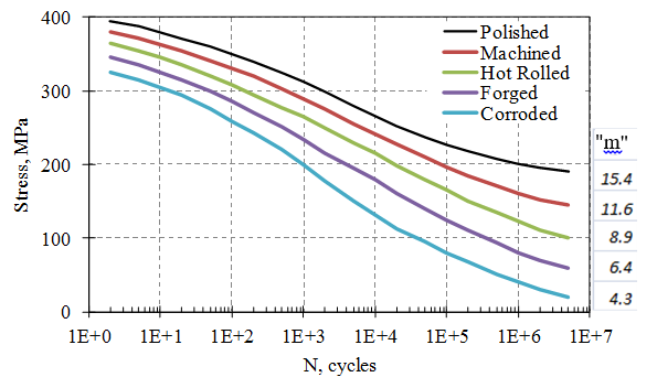
Figure 7. Dependence of Power Variable “m” on Surface Conditions for AISI 1020 Steel
The value of “m” used in Eqs. (5) and (8) must be obtained from the S-N curve for the failing material in its installed condition. Fig. 7 illustrates the dependence of “m” on a variety of surface finish conditions for AISI 1020 steel.
MIL-STD-810G (2008) recommends using a value of m = 7.5 for random vibration excitations. However, a more accurate result for a given product can be obtained by testing a number of units until failure with several different vibration levels and finding the value of “m” that best fits the data.
As an example, Fig. 8 shows tests run on an engine fuel-rail system to determine the fatigue life of the crossover pipe. Shaker tests were run at different vibration levels and the time to failure was measured for each case.
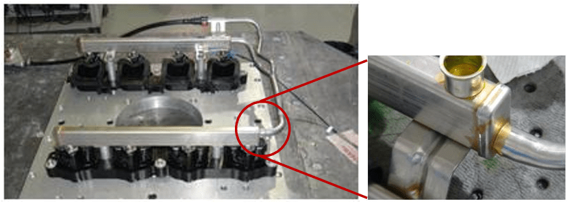
Figure 8. Engine Fuel-Rail System Showing Fatigue Failure at Crossover Pipe Joint
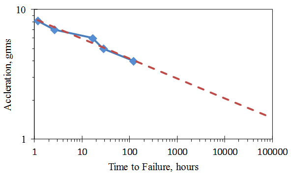
Figure 9. Acceleration-Time Plot of Fatigue Failure Tests on Fuel-Rail System;![]()
Fig. 9 presents the results on an acceleration waveform plot. A curve fit to the data gives a value of m = 6.5. (Note: since the curve fit is exponential, the scale factors to convert acceleration to stress and time to cycles do not affect the value of m.)
A fatigue test can then be accelerated by scaling the PSD of the base vibration level using the power law of Eq. (8). The main limitation of this test method is the assumption that the response PDF is Gaussian. Therefore, the only way to accelerate the fatigue test is to increase the overall RMS level of the excitation. This may not be realistic or feasible. This is addressed in the third and fourth test methods below.
3. Accelerated Test Method Using the Fatigue Damage Spectrum
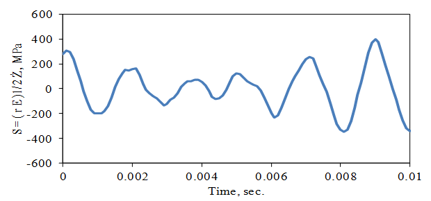
Figure 10. Resonance Response to Random Base Excitation
In many cases, the vibration environment is more complicated than a simple sinusoid or Gaussian random, as was assumed in the previous test method. Also, the vibration and stress levels of the resonances of components in the product being tested may not be measurable. In these cases, the time history of the stress associated with resonance is simulated using a resonant filter specified by a natural frequency, fn, and a quality factor Q = 0.5/z. This is illustrated in Fig. 10.
In this illustration, the base acceleration is random and broadband in the frequency range. The resonant filter response (assumed to be proportional to the velocity and stress response of a structural resonance) is random in amplitude but narrow band in frequency, vibrating mostly at the resonance frequency, fn.
The failure analysis, in this case, is based on the theory for cumulative fatigue damage developed by Palmgren (1924) and Miner (1945), which assumes a linear relationship between the number of cycles at particular maximum stress and the percentage of damage it causes (where 100% damage results in fracture). If K different stress cycles are applied, each ni times with maximum stress Si, then the total fatigue damage, FD, is given by where Ni is the number of cycles to failure at stress Si on the S-N curve. A value of FD = 1 is assumed to cause failure (which works well for HCF cases).
Lalanne (1984) used the Palmgren-Miner rule, Eq. (9), to evaluate the relative fatigue damage of each potential resonance in a structure. Using the example in Fig. 10, the resonance stress peaks are identified using a method such as the rainflow technique [e.g. Downing (1982), ASTM (2005)], as illustrated in Fig. 11. Each successive traverse from peak to peak is considered to be twice the peak stress magnitude, Sfn, of a half cycle at frequency fn.
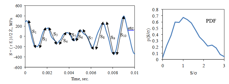
Figure 11. Stress Traverses in Random Resonance Response
The stress cycles are accumulated into a PDF of stress peak magnitudes at frequency fn, denoted by p(Sfn). Over a length of time, t, the number of fatigue cycles at frequency fn is n = fn t, and Eq. (9) can be converted into an integral of the form where Eq. (2) has been used for N with m = -1/b. FD(fn) is called the fatigue damage spectrum, FDS, because it is a measure of the relative fatigue damage as a function on frequency. It measures the amount of fatigue damage a particular base vibration excitation will do to a potential resonance in the product at frequency, fn, (with a damping ratio of ζ).
Henderson and Piersol (1995) evaluated the FDS for the case of a Gaussian random vibration response using results from Crandall and Mark (1963) showing the PDF of the stress peaks will have a Rayleigh distribution of the form where σ is the standard deviation of the stress time history. Using Eqs. (6) and (7) to convert the stress levels to vibration levels the FDS becomes
 where c’ is a constant. Taking the ratio of Eq. (12) for two different values of W(fn) gives the same result as Eq. (8), as expected for the Gaussian response distribution. But the formula of Eq. (10) can be used to evaluate the FDS for any non-Gaussian vibration environment.
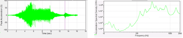
Figure 12. Measured Time History and Frequency Spectrum of Engine Head Vibration
As an example, consider the measured engine head vibration level, shown in Fig. 12, which is considered to be the base vibration for the fuel-rail system shown in Fig. 8. The specifications for the fuel-rail system require it to survive this excitation level for 120 hours.
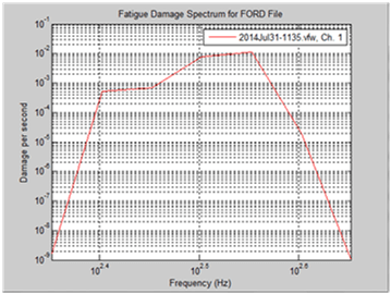
Figure 13. Fatigue Damage Spectrum Computed from Measured Engine Head Vibration
Using a rainflow algorithm, the FDS is evaluated as shown in Fig. 13. In this case, the FDS is calculated as a relative level per unit second. Since the value of m was determined from fatigue tests to be 6.5 (see Fig. 9), the relative scaling of a vibration amplitude waveform can be determined to maintain the same fatigue damage. For example, if it is desired to reduce the length of the endurance test time from 120 hours to 16 hours (a factor of 7.5), the linear amplitude of the signal need only be increased by a factor of (120/16)(1/6.5) = 1.36.
This example assumes the PSD of the excitation signal remains unchanged as it is scaled up to reduce the test time. The next test method allows for an endurance test time to be reduced even more by changing the PSD in a controlled manner.
4. Accelerated Test Method Using Kurtosis Control
Henderson and Piersol (1995) noted that shakers using periodic, impulsive excitations can sometimes give non-Gaussian vibration responses in structural resonances. This can be seen by considering the impulse response of a resonance, as shown in Fig. 14.
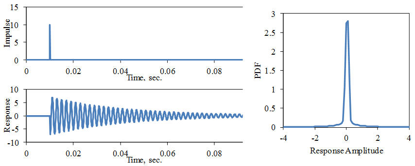
Figure 14. Impulse Response of 500 Hz Resonance, ζ = 0.01, k = 20
The response PDF is very non-Gaussian. One measure of this is the kurtosis, k, (normalized 4th moment) of the response vibration levels. A Gaussian PDF has a kurtosis value of k = 3. The non-Gaussian signal in Fig. 2 has a kurtosis value of k = 6. The kurtosis of the resonance impulse response over time, T, is given by k = 3 π fn ζ T = (3/2) π fn T / Q, where Q = 0.5 / ζ is the resonance quality factor.
If the excitation consists of a series of impulses occurring at a rate of fo = 1/T, as shown in Fig. 15, then the kurtosis is given by k = 3 π ζ fn / fo.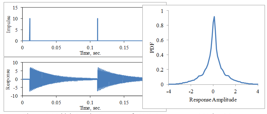
Figure 15. Multiple Impulse Responses of 500 Hz Resonance, ζ = 0.01, k = 5.5If the excitation consists of more impulses at random times and amplitudes, as shown in Fig. 16, then the response PDF begins to converge to a Gaussian distribution as more impulses are contained within the resonance response time constant approximated by τ = 1 / (2 π fn ζ).
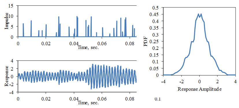
Figure 16. Multiple Impulse Responses of 500 Hz Resonance, ζ = 0.01, k = 3
The patented kurtosis control technique by Vibration Research [Van Baren (2008)] takes advantage of this phenomenon by creating a high kurtosis excitation signal with an adjustable transition frequency setting. This allows for higher stress peaks without increasing the overall RMS of the excitation, thus allowing for shorter test times.
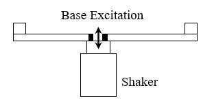
Figure 17. Test Cantilever Beams Constructed with Hot-rolled AISI 1020 Steel.
To illustrate this, two cantilever beams with an accelerometer attached at the tip are driven at the base with a shaker (see Fig. 17). The fundamental resonance frequencies of the long and short cantilevers are 17.5 and 49 Hz, respectively, with damping values of ζ = 0.01. First, the excitation is a Gaussian random signal with an RMS value of 1.0 g and a flat PSD level from 10 to 1000 Hz.
The measured PSD and PDF of the base and tip accelerations are shown in Fig. 18. (Note: the amplitude of the PDF is plotted on a log scale to better view the levels of the tails of the distribution.) The PDF’s of the base excitation and tip response of both cantilevers are Gaussian.
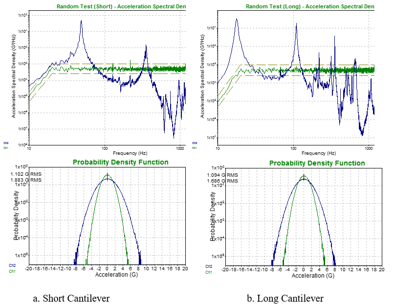
Figure 18. PSD and PDF for Cantilever Responses to 1.0 g RMS, Gaussian Base Excitation. (Green Lines: Base Excitation; Blue Lines: Tip Response)
Next, the excitation uses the patented Kurtosion control signal with the same RMS value and PSD level but with the kurtosis increased to k = 9. The transition frequency is set at 10Hz. The measured PSD and PDF of the base and tip accelerations are shown in Fig. 19. In this case, the long cantilever, with a fundamental resonance frequency of 17.5 Hz, still has a Gaussian response PDF. However, the short cantilever, with a fundamental resonance frequency of 49 Hz, now has a high kurtosis response PDF, similar to the excitation signal.
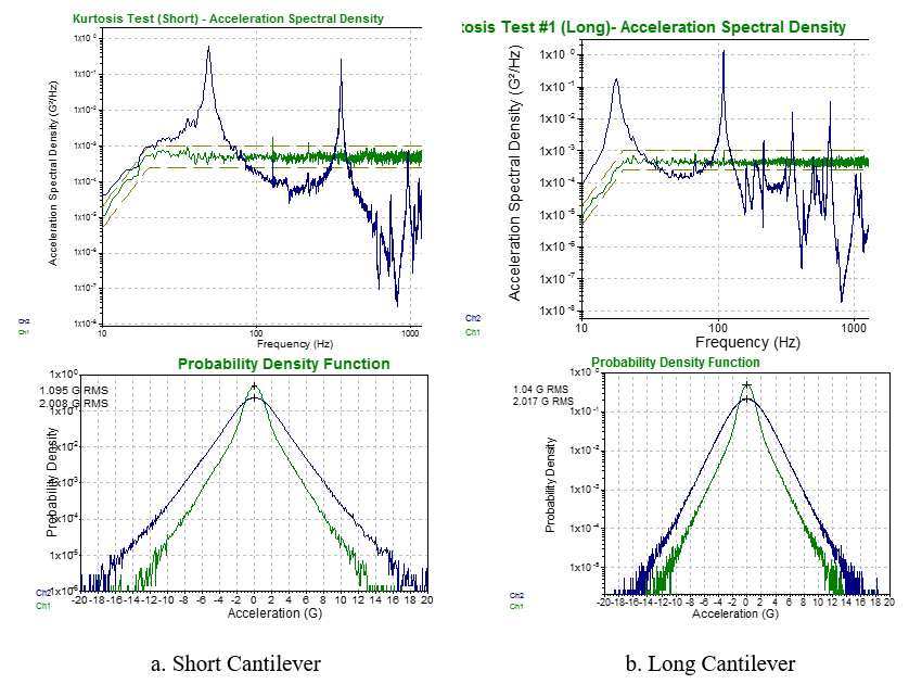
Figure 19. PSD and PDF for Cantilever Responses to 1.0 g RMS, k = 9, Ftr = 10 Hz Excitation. (Green Lines: Base Excitation; Blue Lines: Tip Response)
Finally, the transition frequency is lowered to 2 Hz with k = 9 and the resulting PSD and PDF of the base and tip accelerations are shown in Fig. 20. In this case, the long cantilever now has a high kurtosis response PDF, similar to the excitation signal.
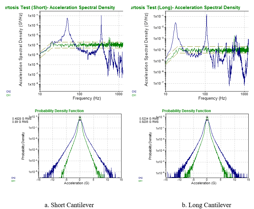
Figure 20. PSD and PDF for Cantilever Responses to 1.0 g RMS, k = 9, Ftr = 2 Hz Excitation. (Green Lines: Base Excitation; Blue Lines: Tip Response)
Furthermore, with a higher kurtosis, the Fatigue Damage Spectrum can be increased without increasing the RMS level of the signal, as shown in Fig. 21. This allows for shorter fatigue testing time without stretching the capacity of the vibration shaker.
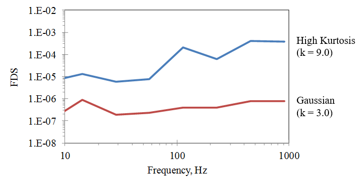
Figure 21. Fatigue Damage Spectrum for Cantilever Resonances (m = 8.0, = 0.01), Base Excitation at 1 g RMS for both cases.
Author: R.G. DeJong (3/20/15), Professor Emeritus, Calvin College, Grand Rapids, Michigan.