University and vocational students nationwide are partnering to take on the three-year Battery Workforce Challenge collegiate competition. Sponsored by the U.S. Department of Energy, this challenge gives students the opportunity to gain hands-on experience in battery design outside of the traditional engineering curriculum. Vibration Research is committed to supporting the next generation of engineers by providing participants with testing solutions that ensure battery durability and safety in real-world conditions.
The following is the culmination of the students’ first year of work, which is provided here for educational purposes only.
Introduction
This report illustrates the mechanical vibration of Ram ProMaster EV’s battery pack. Here, ObserVIEW 2025.1.7 was used to analyze the collected data while driving the EV on a highway and campus road. Then the data was analyzed and plotted to demonstrate the Power Spectral Density (PSD) and Fatigue damage analysis.
Experimental Setup in RAM ProMaster
At first, the five accelerometers were connected to the connector cables, and the cables were connected to the ObserVR1000. Fig. 1 shows one accelerometer sensor connection to the ObserVR1000.
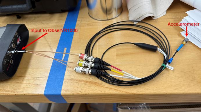
Fig. 1: Sensor connection to ObserVR1000.
Then the GPS was also connected to the ObserVR1000, and the GPS was mounted on the RAM ProMaster for line-of-sight connection to the satellite. Fig. 2(b) shows the GPS mounted to RAM ProMaster [1,2].
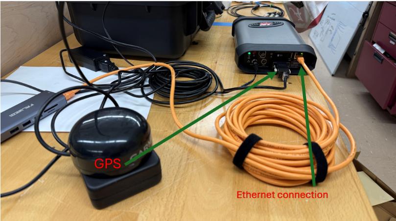
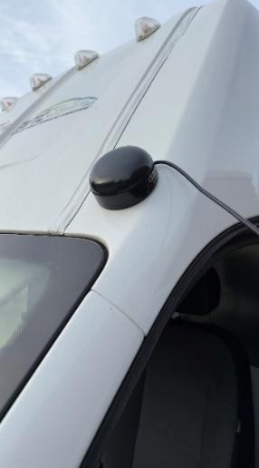
Fig. 2(a) GPS connection to ObserVR1000, (b) GPS mounted to EV.[/caption]
After mounting the GPS, the following Fig. 3 shows the available satellites.
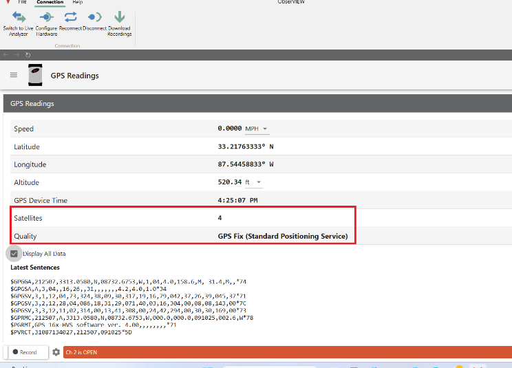
Fig. 3: Available satellites shown in ObserView
Accelerometer Sensor Connection
Now, the five accelerometer sensors are attached to the four corners of the EV, and one in the middle as the diagram shows the positions of the accelerometer sensors considering four corners of the EV battery pack.
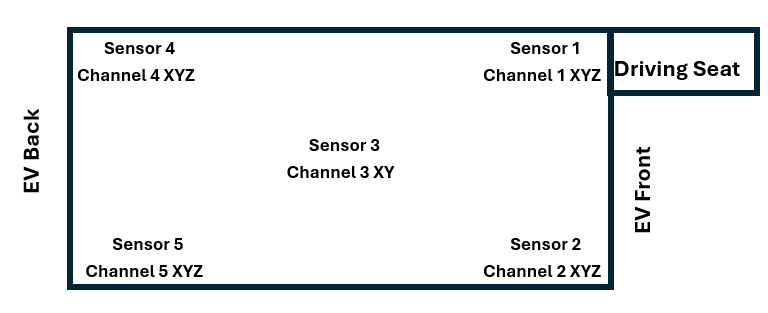
Fig. 4: Diagram showing position of accelerometer sensors.
Fig. 5 below shows the sensors connection displayed in the Obserview software. The Z axis of sensor 3 or Channel 10 was not working while collecting data. All the sensors and wires were attached to EV with double side tape to stick firmly. As there was risk of losing the sensor while driving at road if connected at the bottom of the EV, we considered connecting this inside at five different locations as shown in Fig. 4.
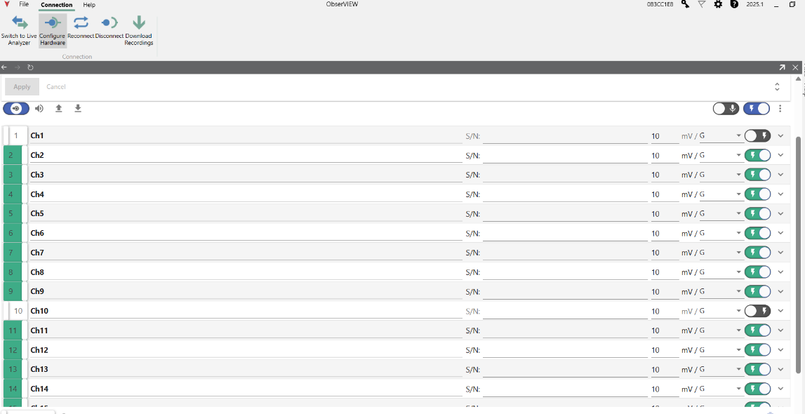
Fig. 5: ObserView window showing channel of accelerometer sensors.
Fig. 6 shows the four accelerometers connected to the different positions of the EV, and these were stick firmly so that it doesn’t move while driving the EV for better data collection. Now, to connect all the accelerometer sensors to the ObserVR100, it was made sure that all wires were not flapping and remain stable as possible. The figures below show four of the five accelerometers’ sensors attached to the different locations of the EV.
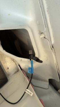
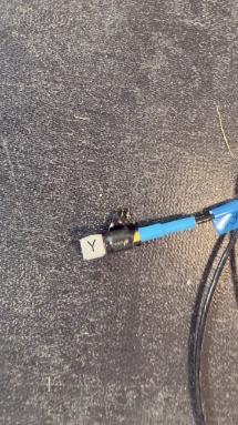
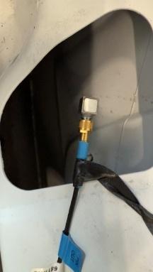
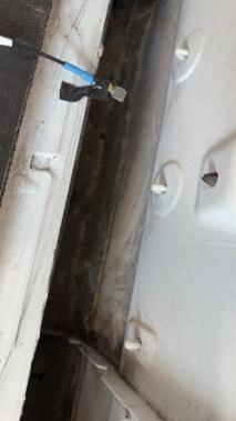
Fig. 6: Accelerometer sensors connected to the corners of EV.
Driving Plan and Route
For the testing, two driving routes have been taken into consideration. For low speed, a set of data was recorded in the campus and city area shown in Fig. 7(a). The Ram ProMaster was driven for almost one mile of 25 miles/hour speed to collect data.
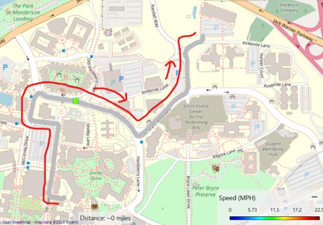
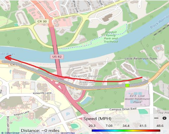
Fig. 7(a): Driving route in campus area, (b) Driving route in highway
Then a set of data was recorded on the highway shown in Fig. 7(b). With higher speed of 50-55 miles/hour. More than two miles were driven to collect data.
Power Spectral Density (PSD) Analysis
The energy distribution of a vibration signal across frequency is described by PSD (Power Spectral Density), which is commonly expressed as  for acceleration. It’s significant since the curve indicates which frequency ranges predominate excitation and integrating the PSD over a frequency band yields the total RMS vibration level. PSD is used to create damage-equivalent vibration tests for durability and to compare actual vibration to standards such as SAE J2380 shown in Fig. 8. The figure shows the standard PSD profile with respect to frequency. The value of the Accelerated Density implies how much RMS acceleration is achieved by an EV with a particular frequency.
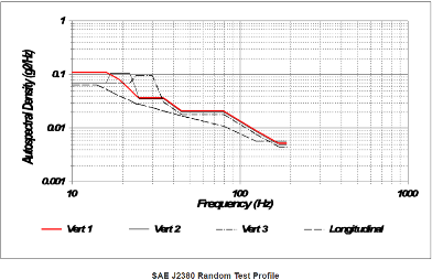
Fig. 8: SAE J2380 standard profile [3].
PSD Graph of Highway
(a) Frequency Band 10-200 Hz
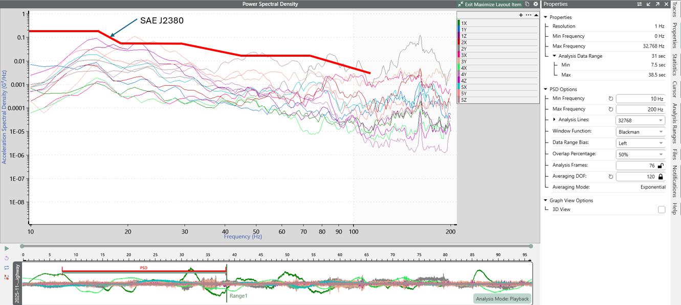
Fig. 9: PSD graph in Highway with low frequency.
From the above Fig. 9, all the five sensors’ data are shown. This figure’s data were taken while driving in highway for two miles. The red marked bold plot shows the standard PSD of SAE J2380 profile. In this figure, the minimum and maximum frequency bands were chosen from 10 to 200 Hz. As SAE J2380 is a specified target input profile rather than a response evaluated on Ram ProMaster vehicle construction, the SAE J2380 PSD curve differs at the beginning. As the frequency increases, the Acceleration Spectral Density of the measured data tends to rise and be similar to the SAE J2380. At 10 Hz, all the sensors’ data are lower than the standard SAE J2380, but when the frequency increases, the Acceleration Spectral Density tends to have less difference with the standard SAE J2380. The roads were chosen relatively smooth for taking caution, it could be the reason as the acceleration spectral density is lower than the standard SAE J2380. At 20 Hz, the PSD curve of measured data seem to have matched the standard profile.
(b) Frequency range 100-1000 Hz in Highway
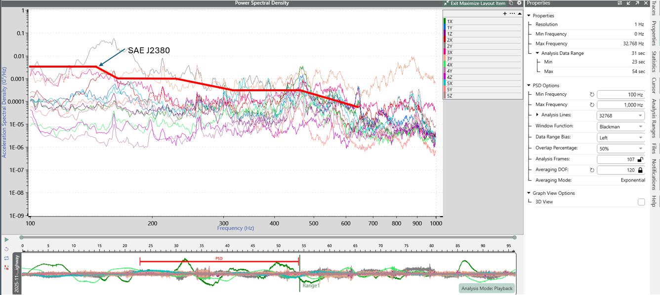
Fig. 10: PSD graph in Highway with higher frequency
This Fig. 10 shows the PSD plot of data taken in highway with frequency range 100-1000 Hz, and red bold marked plot shows the standard SAE J2380 profile. The only difference from Fig. 9 is that this Fig. 10 is plotted with higher frequency. As it can be seen that with the increase of the frequency, the Acceleration Spectral Density is relatively similar to the SAE J2380 standard. As it can be seen that from 100 Hz, all the curves following the standard SAE J2380 graph despite some random peaks. Two passes were driven in highway so that it can be driven enough to follow the standard curve of SAE J2380.
PSD Graph of Campus area
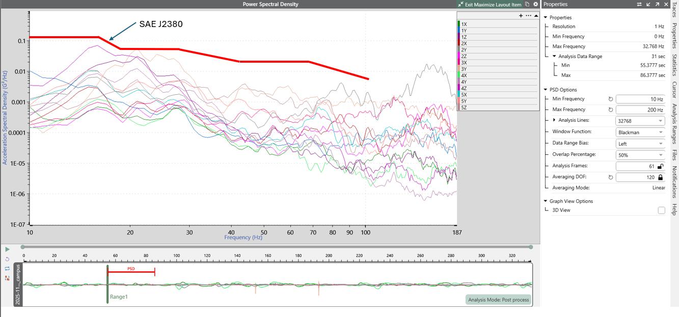
Fig. 11: PSD graph in campus area.
The Fig. 11 above shows the PSD profile for the data of Ram ProMaster while driving in campus area. The frequency range is from 10 Hz to 200 Hz. It can be seen from the figure that the sensors data at low frequency varies from 0.0001 to almost 0.1 . Comparing to the SAE J2380 profile, for frequency range around 22 Hz, the measured data curves show less spike. Despite all the measured graphs are having low Acceleration Spectral Density value of the SAE J2380, the measured graphs follow the decreasing trend over the frequency. These measured values are always below the SAE J2380 curve as the reason might be lower speed of the EV and smooth roads. The SAE profile does not follow the same small-scale frequency changes since it excludes such vehicle-specific resonances. While the observed points might be lower because of suspension, SAE J2380 can stay relatively high to indicate severe road or body excitation in the low-frequency region. Because certain channels couple strongly to resonant elements while others are more isolated, the separation might vary in the mid-frequency band.
Fatigue Damage Spectrum Analysis
The Fatigue Damage Spectrum (FDS) generates an accelerated random test profile that is the damage equal to the relative environment using one or more time-history files. The fatigue damage values that comprise the FDS are computed using the fatigue exponent value (m) value and the resonance factor (Q). Fatigue damage (D) can be described as Miner’s equation (𝑖),
(1) 
Here, 𝑛𝑖 is cycles applied at some amplitude, and 𝑁𝑖 is cycles to failure at that amplitude [4]. By analyzing how a group of single degree of freedom resonators react to the observed vibration input, the Fatigue Damage Spectrum (FDS) illustrates how fatigue damage changes with frequency. The frequency regions where structural resonances would intensify the response and the greatest fatigue damage are identified as peaks in the FDS. Two important parameters are the assumed resonance factor (Q) and the fatigue exponent (m), which regulate resonance amplification and damage sensitivity to amplitude, and have a significant impact on the size and sharpness of these peaks [5]. For the highway driving, Fig. 12 shown below the combined damage spectrum. The overall combined response is represented by the thick blue trace, which illustrates how expected Miner damage changes with frequency for several channels. The blue curve’s peaks show the point with frequency ranges where the vibration input would be most harmful if a component’s resonance is located there, but overall, the damage decreases with frequency ranging from 20 to 2000 Hz. The Q value is 12 and m was taken 5. It can be seen that at lower frequency at 15 Hz, the damage is almost 10% of the total life, but as frequency increases, the total damage is reduced a lot. The following Fig. 13 below shows the fatigue damage spectrum in campus area. It can be seen that, from starting point at 20 Hz frequency the overall fatigue damage is relatively less than the damage in highway driving. This can be due to smooth driving and less vibration of the road. Although there is hump at certain point due to some speed table or braking, other than that the overall fatigue damage shows constant decreasing as frequency increases. The Q and m values are kept constant as in highway driving data analysis.
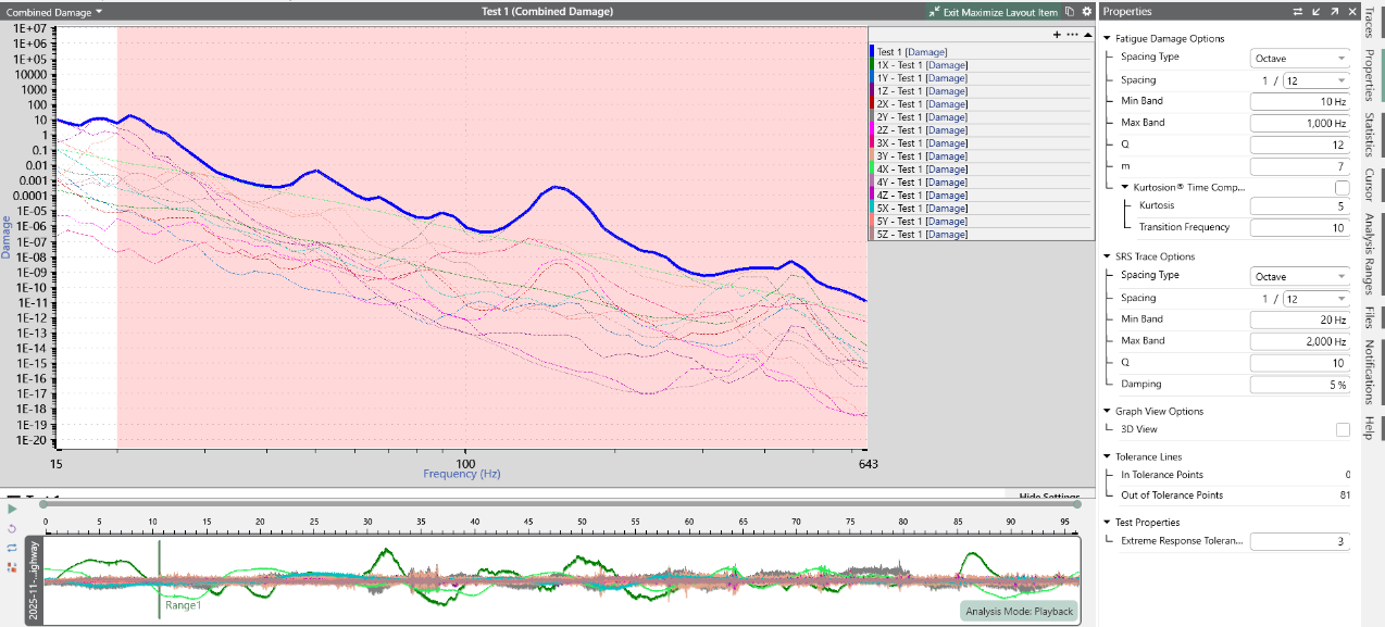
Fig. 12: Fatigue damage spectrum in highway.
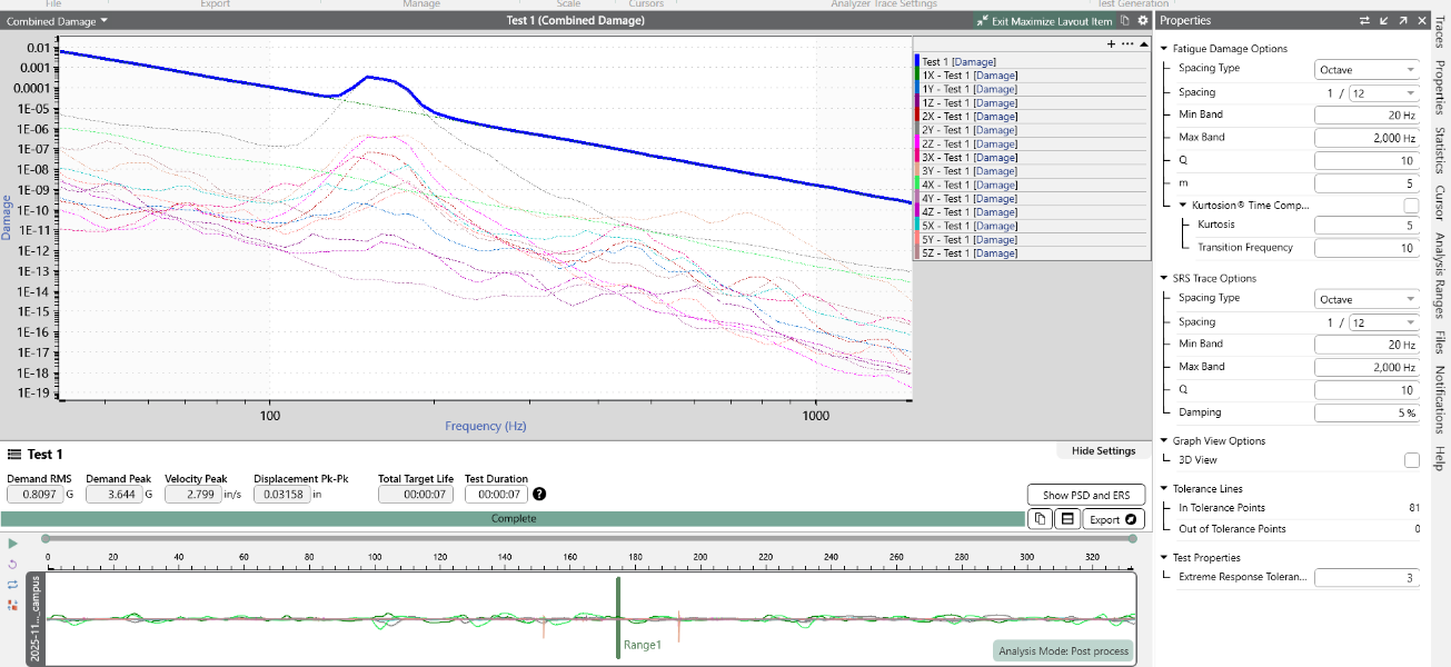
Fig. 13: Fatigue damage spectrum in campus.
Conclusion
The PSD and Fatigue damage response of Ram ProMaster EV have been analyzed here. Because the road and vehicle excitations contain significantly more energy, and large-amplitude motions in very fast vibrations, PSD typically falls with frequency. The EV acts like a low-pass filter, where the suspension, and mounts isolate higher-frequency content while transmitting low-frequency motion. The broadband vibration level tends to decrease as frequency increases due to additional energy dissipation via structural and material dampening. The residual response is frequently restricted to small resonance peaks riding on a declining background at higher frequencies.
From the above analysis, it is our assumption and anticipation that suspension dynamics and vehicle body motion dominate low frequencies. From frequency bands ranging from 0 to 100 Hz as shown in the figures above, several curves start to exhibit bumps or peaks, indicating the beginning of structural resonance influence. Since J2380 is a target environment rather than a particular vehicle structural response, it is smooth and does not exhibit abrupt resonant bumps, while our recorded data varies because of the proper sensor positioning and driving routes.