UNLV CSN Battery Challenge Vibration Measurements and Accelerated Testing
The document TG-2.1.1 gives the following locations on the battery pack for accelerometer placement:
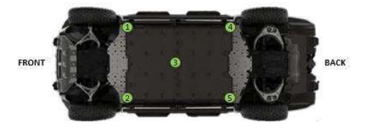
Figure 1. Locations for accelerometer placement from TG-2.1.3
Small 1” x 1” square pieces of aluminum plate were cut and small holes for bolting the accelerometers were drilled into each piece. Gorilla Super Glue was used to set the accelerometer into each plate along with the tightening of the small screw.
Figure 2. Gorilla Super Glue
After the glue was dry, each aluminum piece with an accelerometer and screw was installed in the locations shown in Figure 1. Each location’s surface was cleaned with a small towel with isopropyl alcohol. The underside of the aluminum pieces were glued to the cleaned surface. The accelerometer cables were fed through an existing opening in the floor of the vehicle and connected to the Vibration Research ObserVR1000.
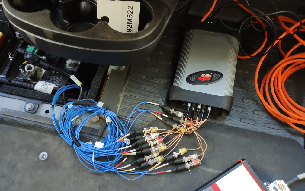
Figure 3. Accelerometer hardware connections.
Here are the accelerometer serial numbers, their locations, and their orientation data labels:
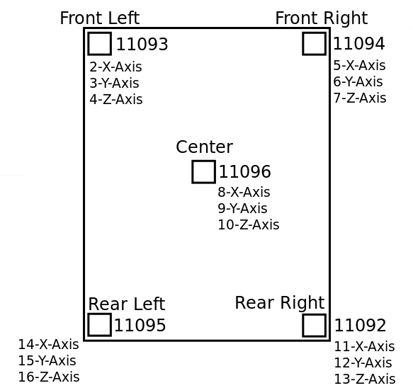
Figure 4. Accelerometer locations, serial numbers, and their data labels.
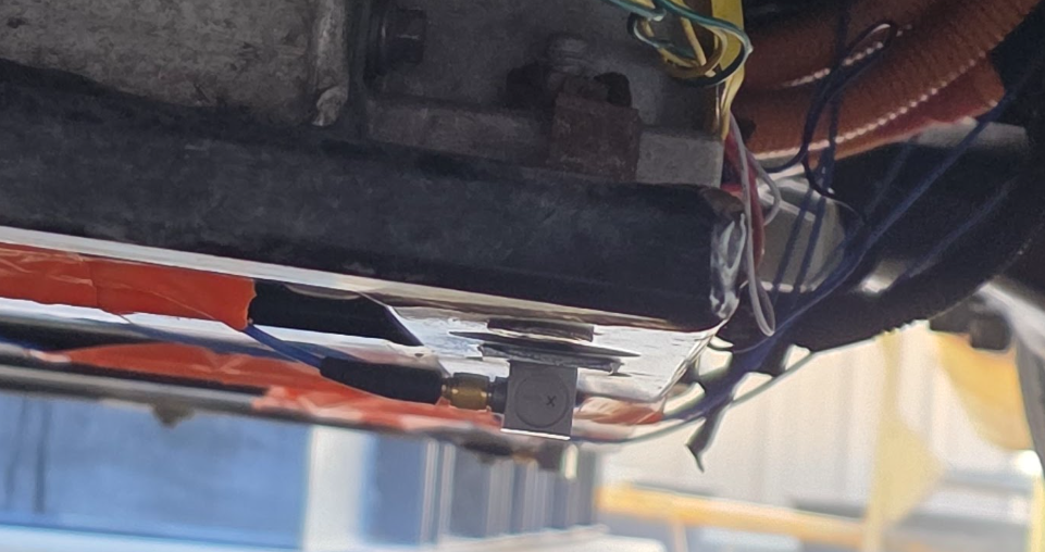
Figure 5. Front Right accelerometer mounted to vehicle.
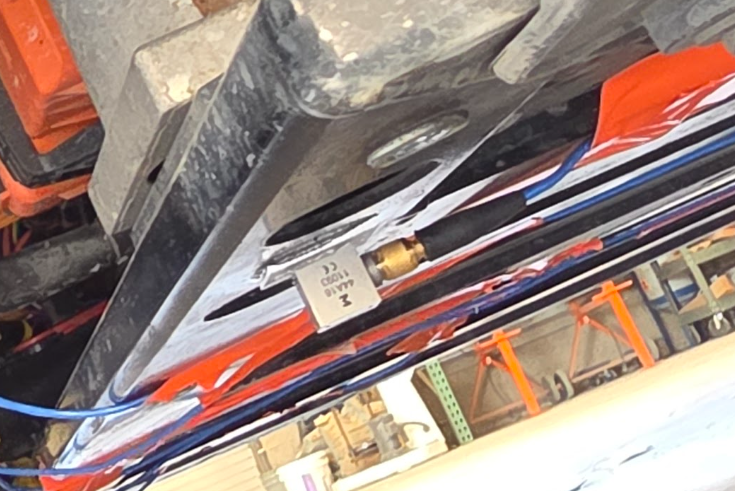
Figure 6. Front Left accelerometer mounted to vehicle.
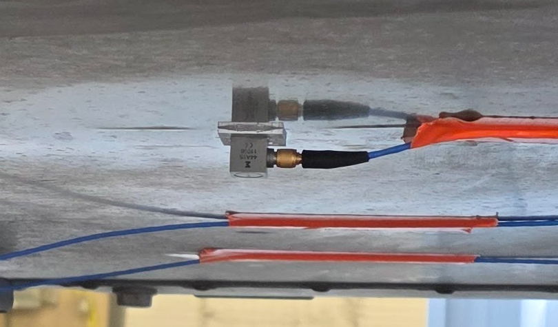
Figure 7. Center accelerometer mounted to vehicle.
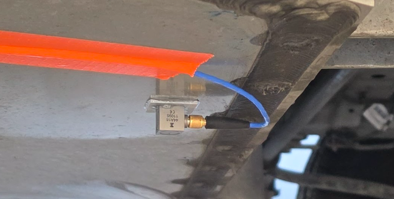
Figure 9. Rear Left accelerometer mounted to vehicle.
Route and Speeds for Measurement Profile
The default sample rate of 65,536 Hz was selected. This high rate should be more than adequate to accurately measure any events experienced. The route taken consisted of 44.3 miles. Several of the roads were fairly rough due to ongoing construction including Maryland Parkway, parts of Las Vegas Blvd, and parts of East 215. The speeds ranged between stop and go due to heavy traffic areas up to 70 mph.
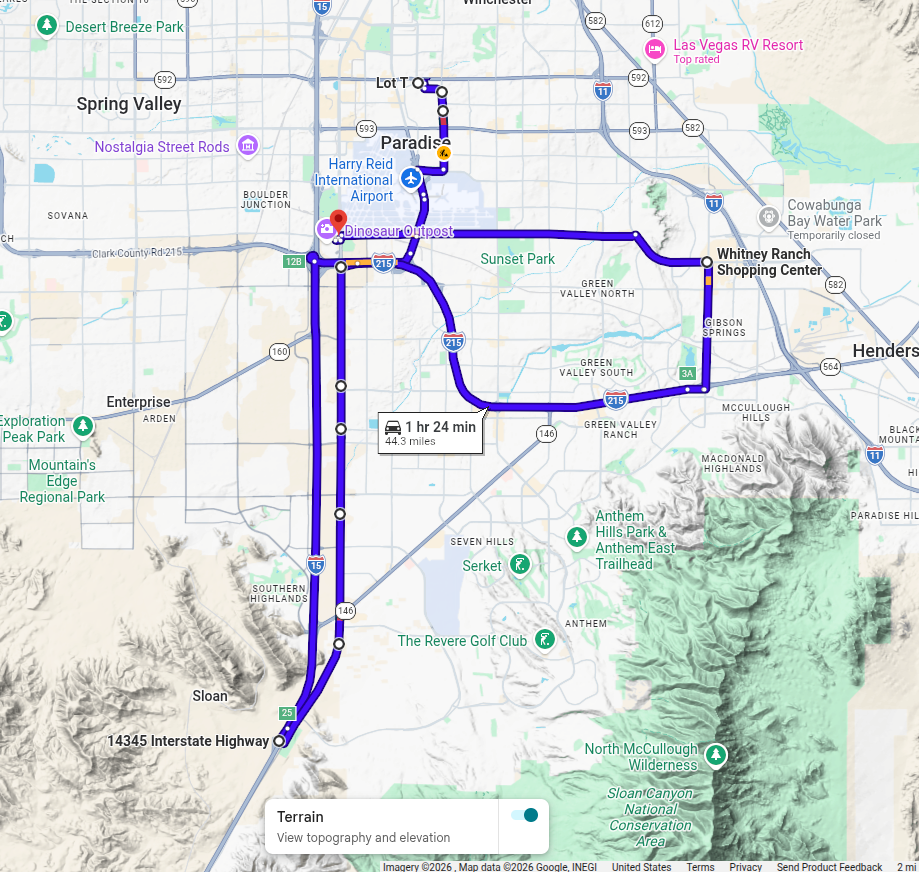
Figure 10. Route taken from UNLV to Tesla Charging Station.
PSD Profile Development
The route consisted of a total distance of 44.3 miles. The entire route was assumed to be a typical daily routine and the number of life passes was calculated by taking 200,000 miles and dividing that by 44.3 miles which is 4,515 life passes (note: an incorrect total distance of 35 miles was used initially which led to using 2,857 life passes for 100,000 miles and 5,714 life passes for 200,000 miles, Figures 11-20 reflect this incorrect value. Figures after this use the correct value). The settings described in the “Field Data to Vibration Profile With FDS” link were mostly used. A 2 Hz high pass filter was applied to the entire data set and two anomalies were removed (extremely square wave two cycles of x10^20 G and an extremely high reading on one sensor and not seen at all on any of the other sensors).
The following settings were used:
Octave Spacing: 1/12
Min Band: 8 Hz
Max Band: 2000 Hz
Q: 10
M: 4
Kurtosion Time Compression: Unchecked (initially)
SRS Trace Options
Octave Spacing: 1/12
Min Band: 8 Hz
Max Band: 2000 Hz
Q: 10
Damping: 5%
Extreme Response Tolerance Multiplier: 3
A profile was made for each axis with a target of 2 hour runtime. Each accelerometer’s axis was combined into a group using the ENVELOPE setting.
Figure 11. X-Axis Profile – 100,000 Mile, 2 Hour Target Runtime
Figure 12. Y-Axis Profile – 100,000 Mile, 2 Hour Target Runtime
Figure 13. Z-Axis Profile – 100,000 Mile, 2 Hour Target Runtime
Comparison with SAE J2380 Profile
The following plots compare the profiles developed from the measured data with the given SAE J2380 profiles.
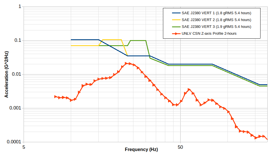
Figure 14. Comparison between SAE J2380 vertical profiles and UNLV CSN Developed vertical profile.
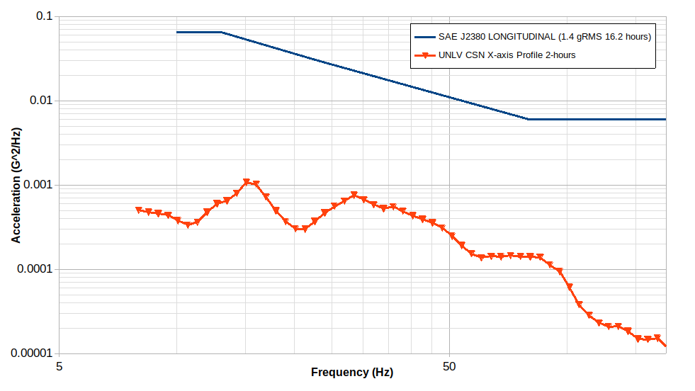
Figure 15. Comparison between SAE J2380 longitudinal profile and UNLV CSN Developed X-axis profile.
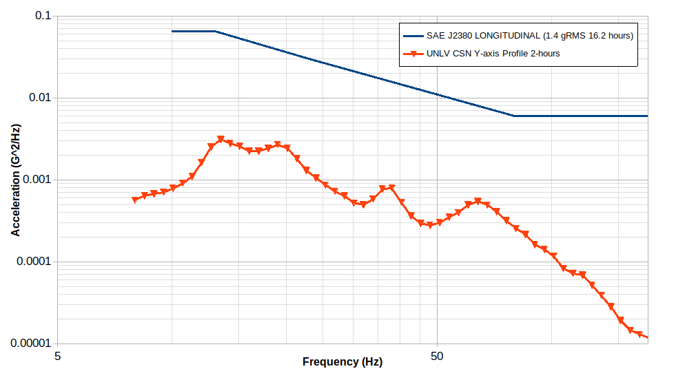
Figure 16. Comparison between SAE J2380 longitudinal profile and UNLV CSN Developed Y-axis profile.
Profiles at 200,000 miles, with Kurtosion Time Compression, and same Target Runtimes as SAE J2380 profiles
Three new profiles were produced to compare with SAE J2380 profiles. The vertical profile targeted 5.4 hours, 5714 life cycles (to be equivalent to 200,000 miles), and Kurtosion Time Compression was used with a Kurtosis of 5 and Transition Frequency of 10.
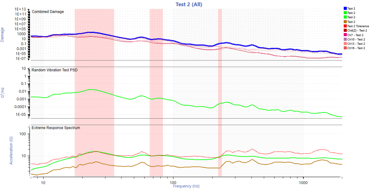
Figure 17. Z-Axis Profile – 200,000 Mile, 5.4 Hour Target Runtime, with Kurtosis
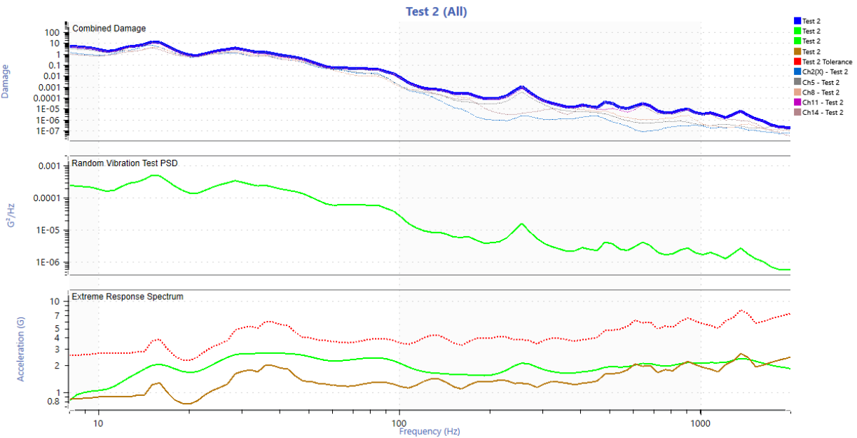
Figure 18. X-Axis Profile – 200,000 Mile, 16.2 Hour Target Runtime, with Kurtosis
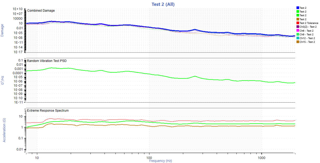
Figure 19. Y-Axis Profile – 200,000 Mile, 16.2 Hour Target Runtime, with Kurtosis
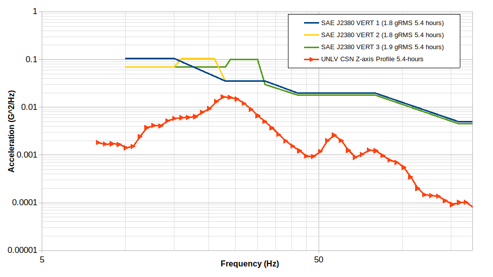
Figure 20. Comparison between SAEJ2380 vertical profiles and UNLV CSN Developed vertical profile at 200,000 mile, 5.4 hour runtime, and Kurtosis.
Very little difference was observed between the two UNLV-CSUN developed vertical profiles so the difference between them and the SAE J2380 profile were not due to number of life cycles, Kurtosis, or target runtime.
Using the Correct Value of Miles for Life Cycle
The process was repeated but for using the correct number of miles of 44.3. The calculation of life cycles assumed 200,000 miles, used Kurtosis, and was calculated for a targeted runtime of 2 hours and a follow up runtime which kept the Extreme Response Spectrum below the upper limit.
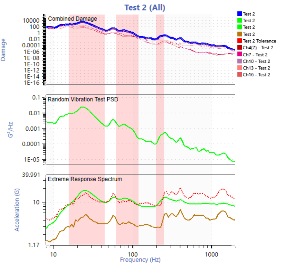
Figure 21. Z-Axis Profile – 200,000 Mile, 2 Hour Target Runtime, with Kurtosis, 4515 LifeCycles
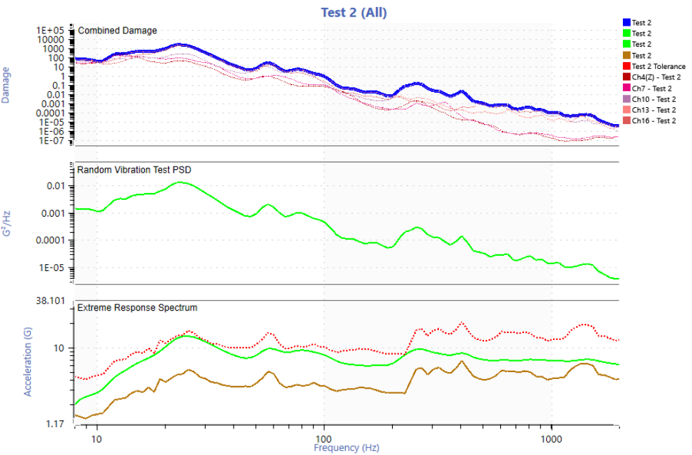
Figure 22. Z-Axis Profile – 200,000 Mile, 7 Hour Target Runtime, with Kurtosis, 4515 LifeCycles
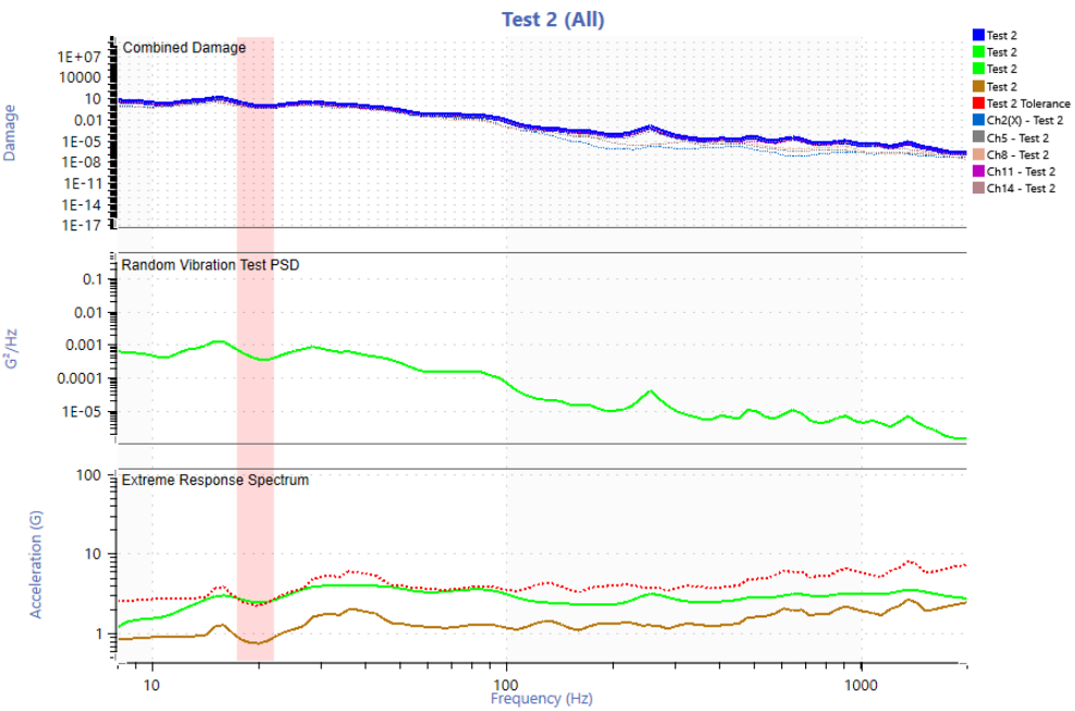
Figure 23. X-Axis Profile – 200,000 Mile, 2 Hour Target Runtime, with Kurtosis, 4515 LifeCycles
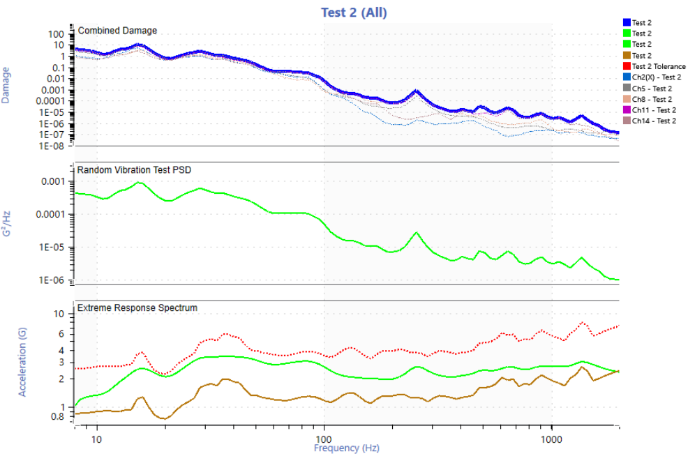
Figure 24. X-Axis Profile – 200,000 Mile, 4 Hour Target Runtime, with Kurtosis, 4515 LifeCycles
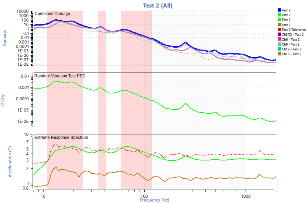
Figure 25. Y-Axis Profile – 200,000 Mile, 2 Hour Target Runtime, with Kurtosis, 4515 LifeCycles
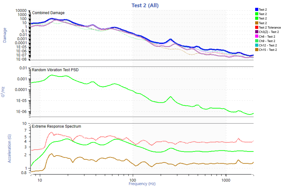
Figure 26. Y-Axis Profile – 200,000 Mile, 6 Hour Target Runtime, with Kurtosis, 4515 LifeCycles
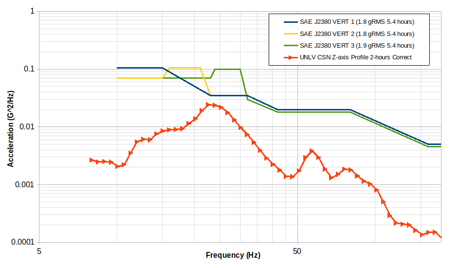
Figure 27. Comparison between SAE J2380 vertical profiles and UNLV CSN Developed vertical profile at corrected life cycle
calculation for 200,000 mile, 2 hour runtime, and Kurtosis.
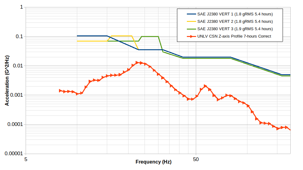
Figure 28. Comparison between SAE J2380 vertical profiles and UNLV CSN Developed vertical profile at corrected life cycle
calculation for 200,000 mile, 7 hour runtime, and Kurtosis.
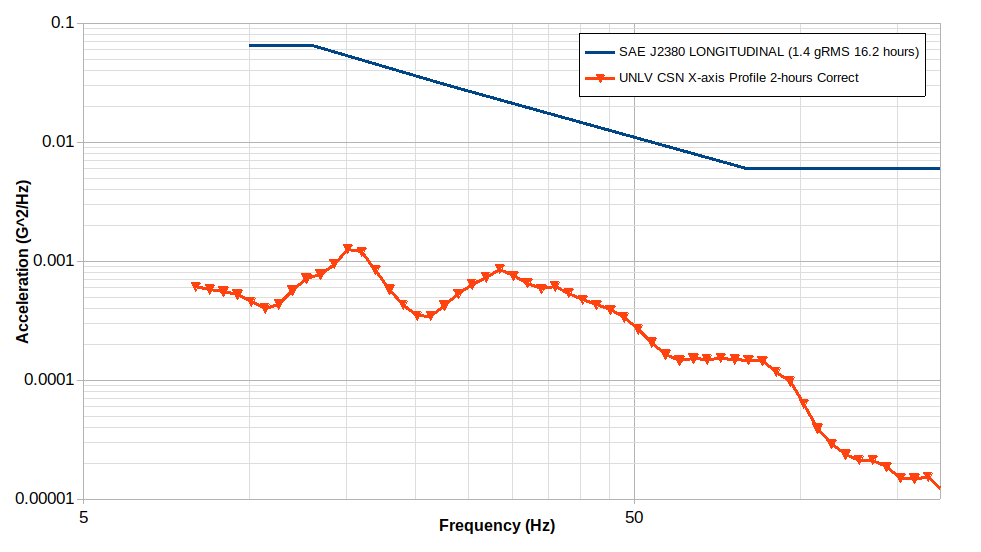
Figure 29. Comparison between SAE J2380 Longitudinal profile and UNLV CSN Developed X-Axis profile at corrected life cycle
calculation for 200,000 mile, 2 hour runtime, and Kurtosis.
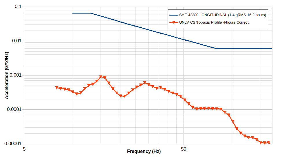
Figure 30. Comparison between SAE J2380 Longitudinal profile and UNLV CSN Developed X-Axis profile at corrected life cycle
calculation for 200,000 mile, 4 hour runtime, and Kurtosis.
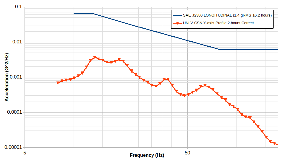
Figure 31. Comparison between SAE J2380 Longitudinal profile and UNLV CSN Developed Y-Axis profile at corrected life cycle
calculation for 200,000 mile, 2 hour runtime, and Kurtosis.
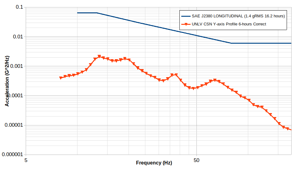
Figure 32. Comparison between SAE J2380 Longitudinal profile and UNLV CSN Developed Y-Axis profile at corrected life cycle
calculation for 200,000 mile, 6 hour runtime, and Kurtosis.
Conclusion
The SAE J2380 profile is more intense than the one developed from field data in Las Vegas. It is suspected that the roads used in Las Vegas may not have been as rough as those used to develop the SAE J2380 profile and/or the vehicle tested had higher shock absorbing capabilities that dampened the shocks felt by the battery pack.