Abstract
Traditional random tests using a Gaussian distribution have not satisfactorily tested products in a realistic manner because the Gaussian distribution method fails to bring into the test the large peak accelerations that cause product failure. The key to bringing those large peak accelerations into the test is to use a random kurtosis control method.
Kurtosion®, the patented technique developed by Vibration Research, is a kurtosis control method that can effectively bring large peak accelerations into the random vibration test. This technique has been criticized by some who appeal to the Papoulis Rule, which indicates that all systems tend toward Gaussian distribution. However, while the Papoulis Rule indicates the output of highly filtered systems tends towards a Gaussian distribution, it does not claim they are Gaussian. Test results obtained at VR with their newly developed kurtosis control technique clearly show that non-Gaussian distributions can indeed be created at product resonances, regardless of the Papoulis Rule.
Introduction
Random vibration testing used today is largely unchanged in technique since it was introduced in the early 1950s. It attempts to capture the essence of the service vibration environment for a product and reproduce a similar environment in the test lab. It does this by summarizing the test environment using a frequency spectrum, which gives the relative weighting of each frequency band, and an averaged overall signal intensity. The frequency spectrum is typically defined as an acceleration power spectral density (PSD), and the overall signal intensity is defined as a root-mean-squared (RMS) averaged acceleration. The primary advantage of random vibration testing, over sine vibration testing, is that random testing produces a waveform similar in appearance to those measured in the field.
However, despite the similarity of random test and environmental waveforms, it is increasingly being recognized that current random test specifications do not capture the field vibration environment with sufficient intensity for many tests. For example, in the automotive world, technicians often see that random tests do not find product faults that should show up when vibration testing. To make random testing more effective, they sometimes take the random spectrum and increase the intensity level according to some formula, such that at the increased intensity level the peak g levels in the random test are closer to those in the original environmental waveform.
Another method to rectify this situation is to use a Field Data Replication (FDR) technique (aka Time Waveform Replication), where the actual waveform measured in the field is reproduced on a shaker in the lab. This method can be extremely useful for many tests. However, critics of this technique claim that since the waveform produced in the test is always the same as one field measurement, it doesn’t capture the variability that can occur in the field. For example, each lap around the track will produce a different vibration waveform, so simply recording a single lap and repeating that lap many times on your shaker removes the variability. Also, the large amount of data involved makes it difficult to define a standard and makes it difficult to define pass/fail criteria for the test. Because of this, there are still very few test specifications based on FDR techniques.
Experience suggests very strongly that the problem with current random techniques is the inability to reproduce the peak accelerations that occur in the actual use of a product. The solution to this problem lies in adding a third control parameter to the vibration tests. Presently, current random techniques are controlled by two parameters – one which controls the frequency content of the PSD spectrum and a second which controls the overall test amplitude (the RMS values). By adding a third control parameter – a kurtosis control parameter – one could control the amount of time the random vibration test runs at higher RMS values. This would provide the desired peak accelerations which cause the real-life product failures that are presently being missed by the current random vibration techniques.
Industry History
Present-day methods of random testing assume a Gaussian mode of distribution of random data. Modern controllers run random vibration tests with the majority of the RMS values near the mean RMS level, thus vibrating the product only for a short time at peak RMS values. In fact, a Gaussian waveform will instantaneously exceed three times the RMS level only 0.27% of the time. When measuring field data, the situation can be considerably different, with peak amplitudes exceeding three times the RMS level as much as 1.5% of the time. This difference can be significant since it has also been reported that most fatigue damage is generated by accelerations in the range of two to four times the RMS level.1 Significantly reducing the amount of time spent near these peak values by using a Gaussian distribution can therefore result in significantly reducing the amount of fatigue damage caused by the test relative to what the product will experience in the real world.
This Gaussian distribution has been in use since the infancy of random vibration testing and continues to be used in the present-day industry for several reasons. First, linear filtering of one Gaussian distribution will result in another Gaussian distribution, so spectrum shaping and the shaker frequency response function do not change the amplitude distribution. Secondly, a Gaussian distribution can be completely determined by two parameters – the mean and standard deviation. In a random vibration context, the mean (the average acceleration) is always zero. Therefore, the Gaussian distribution of a standard random vibration test can be completely defined using a single parameter – the standard deviation (the RMS acceleration). Gaussian distribution is used, therefore, because of its simplicity.
A Better Method than the Gaussian Distribution—Kurtosis
To understand a new method that can be used to improve upon Gaussian distribution, it is important to review the meaning and significance of a statistical term – kurtosis. Kurtosis is a statistical term used to describe the relative distribution of data, similar to RMS. Note that the RMS value of a waveform is the square root of the second statistical moment. Normalized Kurtosis is defined as the ratio of statistical moments. Normalized kurtosis is defined as the fourth statistical moment divided by the square of the second statistical moment. This normalization is done to remove variability due to waveform amplitude from the measurement. In this normalized form, the kurtosis for Gaussian data is always 3, regardless of the RMS level or PSD. The normalized kurtosis value k can be computed from N samples of zero-mean waveform data, xi, using Equation 1. If your data is not zero-mean, you must subtract off the mean prior to the above calculation.
(1) 
Graphically speaking, kurtosis is a measurement of the size of the distribution’s “tails”. A set of data with a high kurtosis value will produce a distribution curve with a higher peak value at the mean and longer “tails”, or in other words, more data points at the extreme values from the mean (Figure 1). In fact, the kurtosis value is sometimes also referred to as the ‘peakiness’ factor.
Now consider the probability distribution of a random test. The Gaussian distribution, with a kurtosis of 3, fails to reproduce the same peak levels seen in field data. We have seen that kurtosis is an indication of the peakiness of the data, and as such, is a desirable parameter to include in the random controller to better match the PDF of the field data. In fact, it may even be a required parameter for a random test to be realistic.
Therefore a better method of testing products than using the Gaussian distribution of data is to adjust the distribution of data to more closely fit the real-world data by adjusting the kurtosis level. The difference between the Gaussian distribution and a distribution with a higher kurtosis value is simply the amount of time spent at or near the peak levels. Adjusting the kurtosis level to match the measured field level will result in a more realistic test.
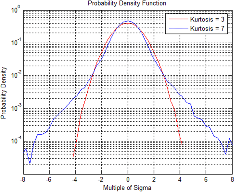
Figure 1: A comparison of kurtosis values 3 and 7. Note how the higher kurtosis value includes higher sigma values (higher peak accelerations).
Criticisms
Two of the key causes of product failure are large peak accelerations and the presence of resonances in the product. Traditional random tests, using the Gaussian distribution, do not satisfactorily reproduce large peak accelerations. Kurtosion™ is a closed-loop method of kurtosis control that can test a product in a more realistic manner by including these larger peak accelerations. However, the method of kurtosis control occasionally comes under fire because some, citing the Papoulis Rule2, claim that regardless of what input is sent to the device under test (DUT), at the resonance frequencies of the DUT the filtering inherent in resonance will result is a vibration that is Gaussian.3,4 The basis of this criticism is that regardless of how many large peaks (and resulting in higher kurtosis) are programmed into the test, the product resonances act as low-pass-filters, and this filtering will average out the peaks to make the data more Gaussian. As a result, it is argued that even if the shaker motion has a high kurtosis level, the product will have a Gaussian distribution because of the averaging inherent in the resonance. Therefore the critics believe that the kurtosis control process is invalid, as they assume, using the Papoulis Rule for support, that regardless of the kurtosis value produced on the shaker, the resulting vibration on the product will always be a Gaussian distribution.
Papoulis Rule
To properly understand these criticisms and where they go wrong, it is necessary to make a brief examination of the Papoulis Rule2. The result in the Papoulis paper creates a bound on the difference between the cumulative distribution function (CDF) of the output of a narrowband filter and that of a Gaussian distribution and then proves that this bound goes to 0 as the bandwidth of the filter goes to 0. Therefore Papoulis’ Rule (and the Central Limit Theorem) proves that the output of a narrow band filter tends towards Gaussian, not that it is Gaussian.
Looking closely at the bound, we also see that the bound is proportional to ω0 (1/14) (i.e. the 14th root of the filter bandwidth). This is an extremely weak limit. Also, we note that the bound is constant across all values of the CDF. Since the tails of the distribution are typically already very small numbers, this bound is further weakened in the tails of the distribution. And, since the kurtosis is very sensitive to the tails, the bound must get very small before it brings the kurtosis back to the Gaussian value 3. The practical result of this is the kurtosis at the resonance gets reduced from the kurtosis of the excitation signal, but for practical Q factors, there will still be some significant kurtosis at the resonance. Only for unrealistic Q factors on the order of 1010 or more do the limits really start to take effect. In fact, since the Papoulis Rule defines how narrow the bandwidth for a given waveform needs to be for things to be “close to Gaussian”, we can turn the limit around and learn something else important that Papoulis teaches. For a given resonance bandwidth and the desired deviation from Gaussian (i.e. kurtosis level), one can use the Papoulis Rule to determine what the input waveform needs to be (i.e. the “transition frequency” parameter) to ensure the result is still non-Gaussian at the resonance.
Demonstrating the Ability to Produce Non-Gaussian Outputs
Vibration Research Corporation has already demonstrated that some real-life data is nonGaussian, demonstrating the need for kurtosis control and that Kurtosion™ can bring the large peak accelerations into the random vibration tests – something traditional non-Gaussian methods can not do.5,6 What remains to be demonstrated is whether or not the kurtosis control can generate the large peaks that are found in the real-life data even on the product at the resonant points. Others7,8 have proposed non-linear methods of kurtosis control which lack a key aspect to their methodology, therefore producing Gaussian output as predicted by the Papoulis Rule. Our kurtosis control method, however, has a unique feature to its kurtosis control which produces a non-Gaussian output which allows you to achieve higher kurtosis even at the resonances. This unique feature is called, for a lack of a better term, Transition Frequency. A number of tests have been performed which demonstrate that Kurtosion™, and the unique Transition Frequency feature, is successfully able to reproduce those real-life acceleration peaks in its random vibration test, producing non-Gaussian distributions even at the product resonances.
Test 1: Brass Bar and the Transition Frequency
The key to getting the kurtosis into the product resonances is to set the Transition Frequency parameter less than the bandwidth of the resonances in the test. The Transition Frequency determines the “distance” between the waveform peaks. If the waveform peaks are too close together then the filtering effect of resonance will tend to smooth out the signal, resulting in a nearly Gaussian distribution. By spreading the waveform peaks out, the kurtosis can be maintained in the resonances despite this filtering effect. The following experimental data demonstrate that controlling the Transition Frequency is necessary to receive an output kurtosis value that matches the input kurtosis value.
A: Comparison of Shaker Head and Brass Bar Arm
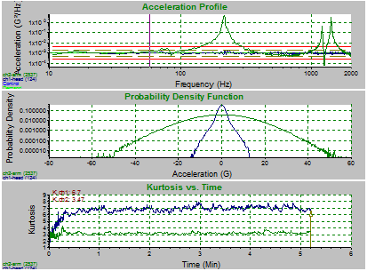
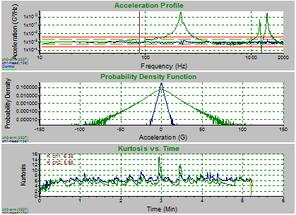
In the first experiment, a brass bar was mounted to a shaker head and accelerometers were attached to each to determine the kurtosis levels of each. A basic random vibration test profile was chosen and the kurtosis for the shaker head was set at 7. The experiment was repeated at different Transition Frequency levels. VibrationVIEW screenshots demonstrate clearly that the random vibration test spectrum remained the same regardless of the Transition Frequency setting. These screenshots also reveal that when the Transition Frequency is high, the kurtosis in the arm is unable to match the controlled kurtosis of the shaker head. On the other hand, when the Transition Frequency is low, the kurtosis in the arm is easily able to match the shaker head kurtosis (Figure 2).
(a)

(b)

(c)
(d)
Figure 2: Screenshot of brass bar random test at transition frequency of a) 10,000 Hz; b) 1,000 Hz, c) 100 Hz, d)10 Hz. Note how the acceleration profiles are exactly the same, but the kurtosis value of the arm begins to match the head’s value as the transition frequency lowers.
B: Comparison of PDFs of Different Transition Frequencies
To look at the same concept from a slightly different perspective, another set of tests was run. A test was run without any kurtosis control (Gaussian) and the resulting data was plotted as a Probability Density Function (PDF). On the same graph were plotted the data from two other trials of data where the kurtosis was set to 5 and the Transition Frequency set to 10,000 Hz in one case and 10 Hz in the other. The PDF shows the probability distribution of the peak accelerations in the test. In a typical Gaussian distribution, the vast majority of the peak accelerations will be within 3 sigma of the average, with only a very few peak accelerations beyond that. Higher kurtosis values will show an increase in the number of peak accelerations at the higher sigma values. This means that higher kurtosis values will include more large peak accelerations than Gaussian will. This is important because these large peak accelerations are the accelerations associated with product failure. In the data set for the brass bar’s arm in this particular study, it is clearly observed that the random test setting in which the Transition Frequency is set to a low value brings about those larger peak accelerations. When kurtosis control has a Transition Frequency set at a very high value the result is not significantly different than a Gaussian distribution (Figure 3.), as predicted by the Papoulis Rule. Therefore, when the Transition Frequency is set at an appropriate level, kurtosis control is able to produce a non-Gaussian output.
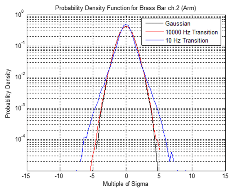
Figure 3: PDFs for the brass bar (arm) data for tests with kurtosis=5 distribution and transition frequencies 10,000 Hz and 10 Hz.
C: Transition Frequency and Resonant Bandwidth Relationship
To see if a direct correlation could be found between the Transition Frequency setting and the resonant bandwidths, a number of tests were run at small frequency ranges centered on a particular resonance. For example, a test was run over the frequency range 1108 Hz to 1308 Hz to capture the 1208 resonant peak of the brass bar (Q= 148, BW=8.1). 16 Transition Frequencies were tested between 10,000 Hz and 2 Hz, including the center of resonance (1208 Hz) and the bandwidth (8 Hz). The results clearly show that the Transition Frequency ought to be set to a value at or below the resonant bandwidth value to bring the kurtosis value of the bar in line with the kurtosis setting of the shaker head (Figure 4). This demonstrates that the Transition Frequency setting is not dependent upon the central frequency of the resonance or on the number of resonances in a particular spectrum, but rather upon the bandwidths of the resonances (Figure 4).
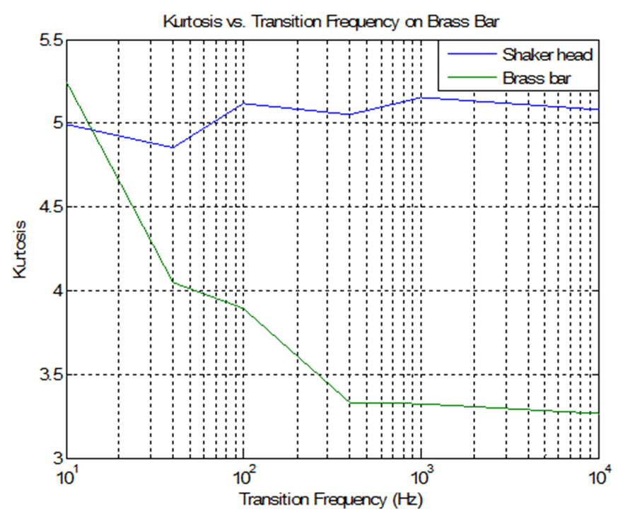
Figure 4: Kurtosis values for shaker head and brass arm vs. transition frequencies for a narrow spectrum band (1108-1308 Hz), incorporating the 1208 Hz resonance peak (bandwidth 8 Hz), demonstrating the kurtosis level can be achieved even at a product resonance.
D: Kurtosis Control and the Transition Frequency
Another test was conducted with the brass bar in which the arm was the control and the shaker head response was observed. A test was run with Kurtosis = 5 in which the shaker head was the control. After the test was run, a new test profile was generated from this test in which the brass bar arm became the control rather than the shaker head. Two test trials were run with this new test profile – one in which the Transition Frequency was very high (10,000 Hz) and one in which the Transition Frequency was very low (10 Hz). This simple test demonstrated that when the Transition Frequency is set very high, the shaker head could not shake violently enough to get the desired kurtosis out on the brass bar’s arm. But when the Transition Frequency was set to a low value, the shaker head would vibrate at the desired kurtosis level and so would the brass bar’s arm (Table 1). This once again demonstrates that the kurtosis can get into the resonances only when the Transition Frequency is adjusted to the resonant frequency bandwidth levels. Again, when the Transition Frequency parameter is properly adjusted the random test’s output will certainly be non-Gaussian.
| Object | Frequency Range | Transition Frequency | Kurtosis Setting | Kurtosis Head | Kurtosis Arm |
| Brass Bar | 10-2000 Hz | 10,000 Hz | 5 | 10.5 | 3.83 |
| Brass Bar | 10-2000 Hz | 10,000 Hz | 5 | 11.0 | 3.38 |
| Brass Bar | 10-2000 Hz | 10,000 Hz | 5 | 10.3 | 3.85 |
| Brass Bar | 10-2000 Hz | 10 Hz | 5 | 4.99 | 5.63 |
| Brass Bar | 10-2000 Hz | 10 Hz | 4.80 | 10.5 | 4.69 |
| Brass Bar | 10-2000 Hz | 10 Hz | 5 | 5.78 | 5.0 |
Test 2: Simulated Resonance Filtering of Field Data
To investigate how the resonance bandwidth affects the kurtosis measured at a product resonance, we took a typical field data recording, passed this waveform through a simulated resonance filter, and computed the kurtosis of the resulting waveform. This will allow us to see how the bandwidth of the resonance affects the resulting kurtosis.
The field waveform used was a recording measured in a vehicle driving down a gravel road. The kurtosis of the original waveform was measured as 5.7. A 2nd-order resonant system response was applied to this, with a resonance frequency of 300 Hz. The Q-Factor, and thus the bandwidth, of the resonance was varied, and the results plotted as kurtosis of the output waveform vs. the bandwidth of the resonances. As can be seen in Figure 5, the kurtosis does indeed decrease as the bandwidth is reduced, with a significant drop was the bandwidth dropped from 10 Hz to 1 Hz (Q factors of 30 and 300, respectively). For typical Q factors of 10 to 100, there is still significant kurtosis even at the resonance. And even for an extreme Q factor of 10,000, the kurtosis still does not get reduced to the Gaussian value of 3. From this, we can conclude that with the filtering can reduce the kurtosis, for real-world data and practical resonance bandwidths and Q factors, the kurtosis is still significant.

Figure 5: Kurtosis measurements of real-world data after filtering through simulated resonances of varying bandwidth, demonstrating a tendency toward, but not reaching Gaussian for reasonable bandwidths.
Test 3: Light Bulb Tests and Transition Frequency
In 2005, Vibration Research Corporation showed the results of a number of light bulb tests that were run under various kurtosis values to determine the time to failure6. A new run of light bulb tests was made to see the relationship between the time to failure and the Transition Frequency parameter setting (Table 2). These results again demonstrate what the brass bar test mentioned earlier demonstrates – that as the Transition Frequency value decreases the kurtosis gets into the resonances, producing the large resonant peaks that cause the light bulb to fail. Again, the random test output is non-Gaussian, and the increased kurtosis at the product resonance can accelerate the product time to failure.
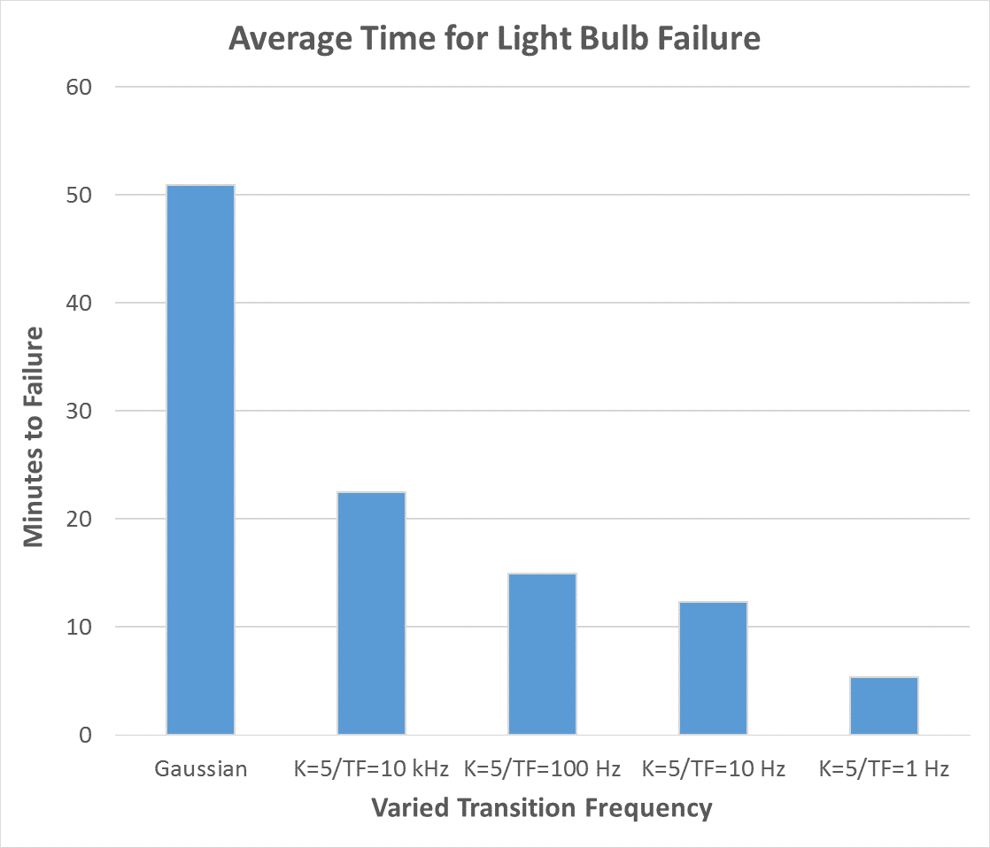
Figure 6: Average time for light bulbs to fail. Note that as the transition frequency decreases so does the time to failure. This demonstrates the effectiveness of the transition frequency parameter at getting kurtosis into the product resonances and producing failures.
| Gaussian 1.00 X RMS |
K=5 TF:10 kHz |
K=5 TF:100 Hz |
K=5 TF:10 Hz |
K=5 TF:1 Hz |
| 32 | 7 | 12 | 6 | 2 |
| 62 | 25 | 12 | 15 | 6 |
| 93 | 30 | 13 | 20 | 8 |
| 102 | 37 | 21 | 24 | 10 |
| 41 | 11 | 10 | 5 | 2 |
| 41 | 13 | 15 | 12 | 2 |
| 45 | 20 | 17 | 13 | 4 |
| 52 | 27 | 19 | 14 | 11 |
| 18 | 19 | 11 | 8 | 2 |
| 36 | 21 | 14 | 8 | 3 |
| 44 | 28 | 15 | 9 | 4 |
| 45 | 32 | 20 | 14 | 10 |
| 50.9 | 22.5 | 14.9 | 12.4 | 5.3 |
Conclusion
These different series of tests communicate the same idea. They demonstrate that the kurtosis control methodology of the patented Kurtosion technique can produce kurtosis in the product, even at the resonances. This result is achieved by adjusting a unique parameter: the transition frequency.
These tests demonstrate that the transition frequency should be adjusted to a level that corresponds with the bandwidth of the resonances present in the DUT to facilitate achieving kurtosis at the product resonance. Papoulis’ Rule notwithstanding, the criticisms that maintain that a non-Gaussian input will always produce a Gaussian output at the product resonance are not valid for this technique. Vibration Research’s unique method of kurtosis control can get the kurtosis into the resonances and produce non-Gaussian output on the DUT, thereby making random vibration tests more realistic.
Get the Slides (PDF)