Abstract
Random vibration control systems produce a power spectral density (PSD) plot by averaging Fast Fourier Transforms (FFT). Modern controllers can set the degrees of freedom (DOF), which is a measure of the amount of averaging to use to estimate the PSD. The PSD is a way to present a random signal—which by nature “bounces” about the mean, at times making high excursions from the mean—in a format that makes it easy to determine the validity of a test. This process takes time as many frames of data are collected in order to generate the PSD estimate and a test can appear to be out of tolerance until the controller has enough data to estimate the PSD with a sufficient level of confidence. Something is awry with a PSD estimate that achieves total in-tolerance immediately after starting or during level changes, and this can hide dangerous over or under test conditions within specific frequency bands, and should be avoided. This paper intends to treat some of the inherent properties of power spectral density estimation, some inaccurate PSD estimation methods that attempt to circumvent these inherent properties, and a PSD estimation method that accurately and quickly estimates the true signal PSD significantly faster than the traditional averaging method: iDOF™.
Introduction
Vibration testing often utilizes the random vibration test. Indeed, because of this test’s ability to simultaneously expose a product to vibrations over a wide range of frequencies at various amplitudes, the random vibration test enables one to gain a comprehensive understanding of the product’s response to vibrations it will encounter in its field of use. This paper concerns the power spectral density of the random vibration test, an integral element in the test engineer’s toolbox.
During a random vibration test, Gaussian time-domain data is transformed into frequency-domain data using the Fast Fourier Transform. Particularly, a set of time-domain samples is transformed into a set of frequency-domain data using the FFT, and having this frequency-domain data the PSD is estimated. Due to the nature of randomness, the PSD estimate generated from one set of sampled time-domain data is volatile, with a high variance between estimated values and the actual PSD value. An effective way to reduce this volatility and decrease the variance between the estimated and actual PSD is to partition the total sampling period into equally-sized time periods (frames), transform the samples from each frame using the FFT, calculate the power of these FFT values, and then average the power values from each set by means of the arithmetic mean. This is generally known as Welch’s method. Hence, this method of FFT averaging requires a noticeable amount of time in order to gather, transform, and average the data, an amount noticeable especially to engineers who wish to know as quickly as possible whether the test and product are and will remain within tolerance limits, since failure to be within tolerance limits may indicate that the test is over-testing and perhaps damaging the product. Several methods of PSD estimation been offered as a solution to this time requirement—attempts to circumvent the time requirement inherent to the PSD—but these lead to inaccuracies, as shown below.
Inaccurate PSD Estimation Methods
Multiplication of Low-Level Data
The most commonly used method involves the multiplication of low-level data. With this method, the controller runs the test on a product at a low level (below demand) while generating and averaging the PSD. The controller uses the averaged PSD of the low-level test, multiplies that averaged PSD by the amount of the level change, and presents the data as if it had been measured at full level—using the results of one test for another. From this starting point, this method then continues averaging. This method is inaccurate because it assumes that the ramped-up data will be a factor-multiple of the lower-level data, thereby assuming that the behavior of the product at a high level would exactly mimic that of the product at a low level. This is not a justifiable assumption, since during changes in level the product being tested cannot be expected to exhibit behavior exactly like that of behavior at a lower level. Further, this method masks the true behavior of the product at a higher level, which undermines the very purpose of a vibration test. This method can mask data so much that, although the PSD generated by this method indicates resonances within tolerance limits, the product being tested may actually be experiencing resonances well outside the abort limits. This method is clearly inadequate and even deceptive. To demonstrate this, a modified NAVMAT test was run on a lawnmower blade, with the control accelerometer positioned near the tip of the blade (Figure 1).
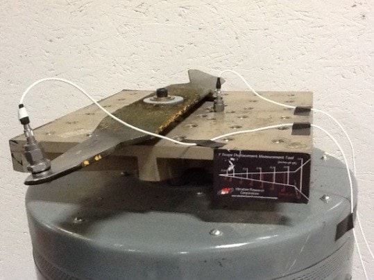
Figure 1: Lawnmower blade on a shaker with accelerometers
The test began at -20 dB (below level) and the PSD estimates were allowed time to converge at that level. Then the test ramped up to 0 dB (full level). The PSD plot produced by a sample controller using this technique had a smooth, low-variance graph when below level (Figure 2) and manifested the same characteristics at full level (Figure 3)—giving the appearance of being within the tolerance limits. But when the PSD plot displayed by the sample controller at level is compared to the PSD plot displayed by a separate signal analyzer measured at the same time using the same signal, it becomes readily apparent that the sample controller is not showing the real vibrations of the lawnmower blade immediately after the transition to full level—it’s simply shifting up the low-level PSD estimates by 20 dB (Figure 3).
Clearly there is a problem. Figure 3 demonstrates that the use of a low-level PSD for a high-level test, although displaying a clean, smooth PSD, nevertheless here is hiding the fact that the product being tested is experiencing large vibrations that are outside of the abort lines. The PSD display of the sample controller here is not reflecting reality, indicating a serious flaw in this methodology. What is happening here is that the resonances in the product are shifting when the acceleration amplitude changes and the controller takes some time to correct for these shifts. It is critical that the engineer be aware of the actual conditions experienced by the product. When the true acceleration levels are averaged in with the factor-multiplied low-level measurements, the fact that full level vibrations are initially well outside of the abort lines is concealed from the user, and the user is left with the false impression of the test being within tolerance.
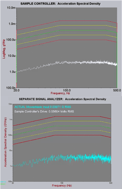
Figure 2: Sample controller PSD at 20 dB below level compared to a separate signal analyzer.
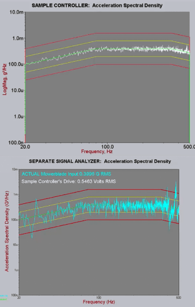
Figure 3: Sample controller at level compared to a separate signal analyzer. Note that the sample controller plot is simply a multiple of the low-level plot. Further, note that the sample controller does not show the resonant peaks truly present in the blade.
Non-Updating of the PSD
Another PSD estimation method designed to ensure a clean, smooth, low-variance PSD display essentially ignores the early-test display of the PSD. Since the variance of the PSD estimate is highest at and near the beginning of the random test—which is normally (and properly) evident in a ragged PSD plot during this time—this method simply doesn’t display the averaged PSD estimate until the variance has been reduced through averaging to a level that neatly falls within tolerance lines. The consequence? The test engineer doesn’t know what’s going on during this time—he or she doesn’t know how the product is behaving. Yet, the whole point of displaying the PSD is to see how the product behaves during a random test. Although the test engineer doesn’t see a ragged PSD, he or she doesn’t seeing anything during this time. This method, too, is clearly flawed.
Appendix 1: Properties Inherent to the PSD
PSD estimation and display require averaging by virtue of what random means. Further, in the early stages of a test, the PSD display should be ragged. Large variance (i.e., raggedness) in the PSD display is expected during this time and indicates the veracity of the test. On the other hand, the absence of large variance in the early stages indicates a problem with the test or the PSD estimation method. To see why, consult Reference [1]:
The PSD of a Gaussian random waveform is computed using a Fast Fourier Transform (FFT). The FFT is a linear transform, and it is given a Gaussian input. As a result, the output of the FFT at each frequency line is a complex number, with a Gaussian real part, and a Gaussian imaginary part. These are squared and added together to get the magnitude, so the square magnitude of the FFT output is a Chi‐squared distributed random variable with 2 degrees of freedom (DOF). To compute an averaged random PSD, F frames of time data are measured, an FFT of each frame is taken, and the square magnitudes are averaged together. As a result, the averaged PSD of a Gaussian waveform is a Chi‐squared-distributed random variable with 2F DOF. [1]
Examining this in the simplest case (without treating overlapping, windowing, and other nuances of the PSD) and supposing Gaussian input data, the PSD estimate at a single frequency bin (without loss of generality)
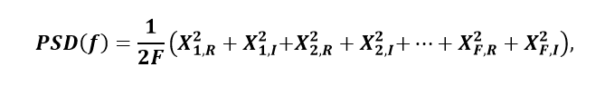
where X2q,R/I refers to the power contribution from the real or imaginary part of the qth frame, and where all the terms are independent and each term is the square of a standard normal random variable. In light of the paragraph quoted above,

The variance of the PSD at frequency bin f
![Var[PSD(f)] = 1/(2F)^2 Var(X_2F^2) = 1/4F^2 4F = 1/F'](https://vibrationresearch.com/wp-content/uploads/2018/08/exploration-psd-estimation-math3.png)
employing the variance property concerning a constant factor and the property that the variance of a chi-square distribution equals twice the number of degrees of freedom involved. Although a simple example, this demonstrates the inherent property of PSD averaging in general that variance is inversely proportional to the number of frames involved in the averaging. Consequently, during the early stages of a test when not many frames of data have been acquired and transformed, the PSD is expected to have and should exhibit high variance. In other words, during the early stages the PSD display is expected to look and should look ragged. If this isn’t the case, something is wrong.
Another concern that has been raised about PSD estimation and the inherent averaging process concerns tolerance limits. While running a random test, why do some lines at times exceed tolerance limits? Consider Table III from MIL-HDBK-340A, Vol. I entitled “Maximum Allowable Test Tolerances” which, for the random vibration power spectral density, states a maximum tolerance of ± 1.5 dB for the 20 to 1000 Hz frequency range. Yet, not every line of a random (and proper) PSD will always be in these tolerance limits for the duration of the test. What’s going on here?
For one, math—specifically, the properties of the chi-square distribution. In Reference [2] states:
Thus we would expect more than 99% of the PSD to be within the ±1,5dB tolerance limit. But we would also expect 0.846% of the PSD to be outside of the tolerance limit. With 800 lines, this means we should expect to see about 6 or 7 lines outside the specified tolerance band at any given time. Also, for 120 DOF the probability shows that only 0.11% of the time will ALL lines be within a ± 1.5 dB tolerance! Ironically, some control systems will consistently show all lines within tolerance for this test when using 120 DOF. The flip side of the statistics, however, tell us that if there are no lines outside the tolerance band, then either the data is not Gaussian, or the DOF is much greater than 120. [2]
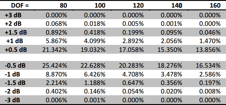
Table 1: Probability of a PSD value exceeding the tolerance dB for a given DOF.
The desire or expectation that all lines in a PSD meet tolerance limits at all times, or that the PSD display immediately (without any averaging time) be a neat, clean, non-ragged, and in-tolerance curve, is unrealistic and asks too much of the PSD estimation, and even more so, asks too much of the math undergirding the PSD estimation. Simply said, the math doesn’t allow it, and if the PSD estimation seems to be exhibiting such behavior one ought to reevaluate the actual test being run or the underlying methodology of the PSD estimation. Or, if a test specification requires every line of the PSD plot to always abide by the tolerance limits—even in the early stages of the test—one ought to reevaluate that test specification. PSD estimation using FFT averaging requires just that—averaging—and averaging takes time. Over time variance will decrease and over time each line will fall in place within tolerance limits (assuming a reasonably tame test and product), but until then there will be volatility in the PSD estimates by virtue of randomness. Reference [3] also treats the PSD estimation’s chi-square statistics, provides tools for statistical analysis of any PSD estimation to see whether it conforms to and abides by chi-square statistics, and provides an example of a controller utilizing more degrees of freedom than was asked for and therefore displaying a misleading PSD.
Reduced averaging
In order to achieve the goal of accurately displaying what is occurring on the product under test, it is then necessary to discard the measurements taken at low level and begin averaging anew once the system has reached full level. This allows the user to see what the true vibration levels are on the product soon after the level transition, without confusing them with the measurements made at lower amplitude levels. These initial measurements will exhibit high variance simply due to the random nature of the test and Welch’s method of averaging. The statistics of the chi-square distribution make this clear. As the test proceeds, more data will be measured and included in averaging the PSD estimates, and those estimates will converge to the actual PSD of the waveform. As that convergence occurs the estimation errors will decrease, the control errors will become apparent, and an appropriate decision may be made as to whether the test is within tolerance.
What needs to be kept in mind is that the high variance of the PSD during the initial stages of the test, or some lines exceeding the abort lines during the initial stages of the test, does not mean there’s something wrong with the PSD estimation method, the actual signal, the test, or the product/shaker response to the drive signal. Such behavior of the PSD estimation is expected—it’s estimating a random signal, and so some volatility is entirely natural, expected, and even desired as verification of the estimation method. Over time, averaging will smooth things out.
Instant Degrees of Freedom
But that’s not the end of the story. Vibration Research has recently introduced iDOF—Instant Degrees of Freedom—a method of PSD estimation designed to rapidly reduce the estimation error at the beginning of a test and after changes in the test level. In doing so, the PSD estimate provided by the iDOF algorithm approaches the actual value of the signal’s PSD quickly, allowing for rapid verification of tolerance limits and/or faster detection of and reaction to an abort condition. iDOF accomplishes this significantly faster than the traditional averaging method. More importantly, unlike other methods, described above, that attempt to rapidly display a clean PSD, the iDOF method produces a PSD estimate which accurately depicts the full level signal PSD, without clouding the estimate with readings made at other test levels. These qualities are evident below.
When it comes to error in the PSD plot (the difference between the control and demand curves), there are two sources: control error and estimation error. Control error refers to the discrepancy between the actual PSD of the data (signal) and the desired demand PSD. Estimation error refers to the discrepancy between the estimated, plotted PSD, and the actual PSD of the signal. For instance, suppose one resets the PSD estimation’s averaging during a test (without changing level). This doesn’t affect the signal, and so the actual PSD of the data doesn’t change, yet the display becomes very ragged until enough new data has been accumulated to average out and accurately estimate the PSD. The error evident in this raggedness is estimation error, since resetting the averaging doesn’t affect the actual PSD of the signal and therefore the error between the actual PSD of the signal and the demand PSD doesn’t change. This is an example where, although the data plotted on the screen has a large variance, the control may be very good, with only a small amount of control error. However, consider the PSD estimation method involving the multiplication of low-level data. During a change in level, the actual PSD of the signal undergoes a major change—including shifts in resonant frequencies—since here the signal is changing (increasing in power). Yet, the inaccurate PSD method doesn’t indicate any changes in the PSD plot during the change in level and at the higher level. During a change in level and at a higher level, although this method gives the appearance of minimal error on the plot, there is a significant difference between the actual PSD of the signal and the estimated PSD shown on the plot. In this case, there are both large control error and large estimation error, and the estimation error offsets and masks the presence of control error.
Estimation error arises from the inherent properties of the PSD as described above, especially from the fact that the PSD estimation is estimating a random signal. Control error concerns the signal and arises from resonances in the signal or other noise added by the system to the signal that takes the controller work to accommodate. It is the control error that interests and is of most concern to the test engineer. Estimation error occurs as a matter of fact when estimating the PSD of a random signal. This estimation error is the 1/F PSD variance described earlier. Even if the signal was perfect, and there was no control error, there would still be an estimation error present in the PSD display, which estimation error would decrease inversely proportionally with degrees of freedom. Further, the presence of estimation error does not imply the presence of control error, since estimation error should not concern the control of the signal.
However, there is a method with which estimation error can be confidently removed, and it is this removal upon which iDOF sets its sights. And iDOF does this in a manner that preserves control error. In other words, iDOF removes estimation error, enabling the user to see control error more clearly.
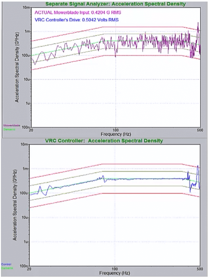
Figure 4: PSD estimated with iDOF at full level compared to a separate signal analyzer
Recall Figure 3 which compares a sample controller PSD plot to that of an independent signal analyzer at full level. The sample controller clearly masked the true vibrations of the mower blade during and after a change in level. Running the same test with iDOF enabled, it is clearly evident in Figure 4 that the resulting PSD estimate preserves and displays the resonances and vibration patterns that the mower blade is actually experiencing (as verified by the independent signal analyzer) while also significantly reducing the raggedness of the plot.
iDOF, in a short amount of time, gives the test engineer a precise view of the signal’s actual PSD, providing a clean, uncluttered picture of the true vibration. Lines that with traditional averaging might have for a time exceeded the abort lines due to estimation error (and not to the signal itself) are quickly reigned in. Yet, when spikes due to resonances or other aberrations applied to the signal by the system are present in the underlying signal’s PSD, these deviations from the demand remain in the PSD estimate and are clearly manifest, as desired, allowing for an appropriate and informed decision as to whether the test is within tolerance, or if a test should be aborted to protect the product.