A graph trace allows you to move a trace cursor over a graph or plot to view the data associated with that point. You can add the trace to the graph for analysis and reporting.
In VibrationVIEW, a math trace displays the result of a math function. The math function is a free entry field that builds a trace using existing trace data operated on by functions and operators.
The software’s math traces feature has two main functions:
- Math function syntax defines a new graph trace derived from standard traces using a math function (15 uses).
- Defining calculators defines a calculation that is computed repeatedly throughout the test, and the results are plotted versus the test time (25 uses).
Math Function Syntax
Equations are written in standard form, and standard math associativity properties apply. For example, (5+3)*2 = 2*(5+3) = 16, but 5+3*2 = 11 and 2*5+3 = 13.
A suite of standard functions is available, including sin, cos, tan, exp, ln, sqrt, and more. You can refer to the appendix for a list of the available functions or check the online Help file.
You can use report fields as calculation variables by enclosing the desired field name in square brackets. For example, [Ch1Accel] displays the channel 1 acceleration. The software implements these report fields as variables, and you can use them anywhere in the equation to replace a numerical value. The square brackets imply a “PARAM” report field, so you do not need to spell out [PARAM:Ch1Accel], although you may.
For a list of available fields, refer to the “How to create customized reports” section in the online Help file or software manual.
Defining New Traces
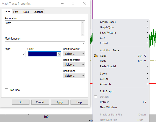 To add a math trace to a graph, right-click on the graph and select Add Math Trace. A dialog box will appear, where you can enter a trace annotation label and an equation.
You can add math traces to nearly any plot and use the plot type to determine the source data. For example, on a spectrum plot, the source data is the channel spectra; on the channel waveforms plot, the source data is the raw waveform traces.
Math Traces Using Time Waveforms
1. Difference waveform
(Ch2 – Ch1)
2. Mark min and max peaks with horizontal lines
Min(control)
Max(control)
Add the math traces “min(Ch1)” and “max(Ch1),” set the line color, and set the line type to a dotted line. Adds dotted horizontal lines to the plot that indicate the level of the min and max values.
3. Displacement time waveforms
disp(Ch1)
Converts the channel 1 acceleration waveform to a displacement waveform with the appropriate unit conversions and trendline removal.
4. Velocity time waveforms
vel(Ch1)
Converts the channel 1 acceleration waveform to a velocity waveform with the appropriate unit conversions and trendline removal.
5. Jerk time waveforms
diff(Ch1)
Differentiates the channel 1 acceleration waveform, which provides the rate of change in acceleration (also called jerk). The units will be the selected acceleration units/second.
6. Differential displacement measurements
disp(Ch2 – Ch1)
DoubleInteg(Ch2 – Ch1)*AtoD
Both of these functions compute the relative displacement waveform between channels 1 and 2, particularly for user-defined transients such as earthquake simulation. The “AtoD” factor converts the acceleration units to displacement units using the configured system unit selection.
The “disp” function removes trendlines due to accelerometer bias to get a 0-mean displacement waveform. The “DoubleInteg” calculation assumes the initial velocity and displacement values are zero. The latter may be more appropriate for transient events that are not necessarily zero-mean but are susceptible to wandering trendlines.
7. Plot the Field Data Replication (FDR) error waveform
Control – Demand
Plots the error signal between the demand trace and control trace in the FDR test mode.
Math Traces Using Frequency Spectra
8. dB error plot in Sine
20*log10(Control/Demand) && (Demand > 0)
Computes the dB difference between the control and demand traces in Sine mode. The logical “&&” operator will only select out the calculations where the demand trace is positive and sets the result to 0.0 where the demand is zero.
9. dB error plot in Random, Shock, or FDR
10*log10(Control/Demand) && (Demand > 0)
Computes the dB difference between the control and demand traces in Random, Shock, and FDR modes. The vertical plot axis is a power value.
10. Weighted average spectrum
(4*Ch1 + 2*Ch2 + 5*Ch3 + Ch4) / 12
Computes a weighted average power spectral density (PSD) of the 4 channels in Random and FDR modes, which have PSD plots.
11. Display the velocity spectrum
vel(Ch1)
Computes the velocity spectrum when the calculation is computed on a frequency spectrum. You can then use the RMS cursor functions to measure the RMS velocity over any sub-band of the spectrum.
12. Display the displacement spectrum
disp(Ch1)
Computes the displacement spectrum when the calculation is computed on a frequency spectrum. You can then use the RMS cursor functions to measure the RMS velocity over any sub-band of the spectrum.
Math Traces Using Histograms (Probability Density Function)
13. Gaussian PDF overlay
exp( -0.5*(x/[Ch1])^2 ) / sqrt(2*pi*[Ch1]^2)
Computes the exact Gaussian PDF trace when provided with the RMS level of channel 1 and applied to a PDF (histogram or amplitude distribution). You can use this trace to compare the actual probability distribution to a true Gaussian distribution.
14. Cumulative distribution
integ(Ch1)
When applied to a PDF, computes the integration of the trace and plots the cumulative distribution function. The cumulative distribution function is the fraction of samples less than the value, so this number will start at 0.0 and end at 1.0.
15. Percent of time above G level
200-100*integ(Ch1+flip(Ch1))
When applied to a PDF, computes the percent of the time that the waveform’s absolute value is above a G level. You should set the Y-axis to log scaling and adjust the X-axis to start at zero; the half of the plot for negative G values will be a mirror image with the addition of 100 percent.
The flip() function reverses the trace and adds the positive values to the negative values to the probability levels for positive values to get the probability values for the absolute value.
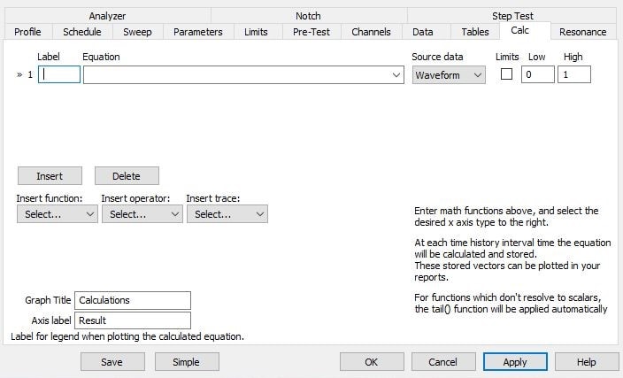
Defining Calculators
The second feature of the math traces is a set of calculators that are computed repeatedly while the test runs. You can define up to 32 calculations on the “Calc” tab in the Test Settings.
The equations are entered the same as math traces, but the stored value is the final value of the vector (highest time sample or highest frequency sample). To control the calculator’s stored value, you can use the min(), max(), mean(), rms(), sum(), integ(), head(), or tail() functions to pick out a specific value.
Each calculator has a selection for the source data: waveform, spectrum, or PDF. You can then plot the calculation versus test time while the test runs using the “Calculator” plot type. You must pre-define these functions prior to running the test, as the software computes and logs the calculation as the test runs. You can add calculations as the test runs, but any calculations you define during a test will only show results after the time it is defined.
Min and max limits may also be defined for each calculator. When the calculation lies outside of the defined limits, the test will abort. This option allows the user to define many different limits. The “High” limit always applies, while the “Low” limit does not apply during ramping up, only at level.
Calculations from Time Waveforms
16. Compute and log the crest factor vs. time
max(Ch1)/RMS(Ch1)
17. Compute and log the peak displacement vs. time
max(abs(disp(Ch1)))
Computes the displacement waveform for channel 1 and then returns the waveform’s maximum absolute value.
Integration from acceleration to displacement amplifies low-frequency noise, so this calculation is susceptible to noise. Additionally, it will fail for low-frequency sine tests where the waveform snapshot does not provide enough of the sine wave to properly integrate.
18. Compute and log the peak jerk vs. time
max(abs(diff(Ch1)))
Computes the jerk waveform for channel 1 and then returns the waveform’s maximum absolute value. The differential of acceleration is the rate of change in acceleration. The units are the selected acceleration units/second.
19. RMS error
RMS(Demand – Control)
Computes the RMS value of the error signal between demand and control from the waveform traces in FDR mode. The RMS calculation will include all frequencies, so this calculation will include frequencies outside of the configured Min and Max Frequency settings.
20. RMS readings
RMS(Ch1)
Provides a short-duration RMS reading. For a spectrum source, it provides a long-duration RMS reading calculated from the averaged spectrum.
Calculations from Frequency Spectra
21. Compute the dB spread of control spectrum
10*log10(max(Control)/min(Control+(1e10*(Demand==0))))
Computes the dB spread of the in-band control spectrum. The 1e10*(Demand==0) effectively removes the out-of-band (zero demand) frequencies from the calculation.
If this factor is omitted, then the calculation is performed over the full band, including the out-of-band noise floor. Random spectra are plotted as power values; to convert to dB, use the calculation 10*log10(ratio).
22. Compute the maximum dB deviation from the demand spectrum
max( abs( 10*log10( Control / Demand ) ) )
Computes the maximum error in dB between the demand spectrum and control spectrum. The max() operator will ignore the infinite values where demand equals zero.
The degrees of freedom (DOF) value determines the smoothness of the spectrum. For example, if DOF=120, we expect 99% of the frequency bins to be closer than 1.6dB. For 800 control lines, we expect eight of the control lines to be greater than 1.6dB at any given time. If you do not have this amount of variation, then your waveform is not truly random. As the waveform is random, it won’t always be the same eight control lines. Instead, they should randomly jump around throughout the spectrum.
23. Compute the number of outlier lines
sum( abs( 10*log10( Control / (Demand + Control*(Demand==0)) ) ) > 1.0 )
Counts the number of spectrum lines more than 1.0 dB from the demand trace. You can change the 1.0 value to the desired dB level for comparison.
24. Compute the average spectrum error, in dB
mean( abs( 10*log10( Control / Demand ) ) )
Computes the average error in dB between the demand spectrum and control spectrum. The mean() operator will ignore the infinite values where the demand equals zero. The average error will be a more statistically stable calculation than the peak error. For Gaussian data, it will directly depend on the DOF value used for averaging.
25. Estimate the DOF from a random spectrum
2*sum(Demand>0) / sum( ((Control-Demand)/Demand)^2 )
The hashiness of the random spectrum for true Gaussian data is directly related to the DOF value used for averaging because the spectrum will also be random with a chi-squared probability distribution with “DOF” degrees of freedom. You can use this relationship to estimate the DOF from the variance of the normalized error between the control and demand spectra.
The sum() operator will ignore any non-finite values. Therefore, this calculation will effectively ignore the graph points where the demand equals zero because they result in a divide-by-0 infinite result.
26. Narrow-band RMS readings
RMS(Ch1*(freq>400)*(freq<500))
Computes the narrow-band RMS of channel 1 between 400Hz and 500Hz. The multiplication of logical (1=TRUE, 0=FALSE) values is a logical and operation. Alternatively, you can use the logical “&&” operator to achieve the same effect.
27. Harmonic levels
RMS(Ch1 * (Freq>(3*[Frequency] – 2.1*df)* (Freq<(3*[Frequency] + 2.1*df) )
Computes the RMS value of the 3rd harmonic for sine tests with spectrum source data. The +/- 2.1*df factor is used because the fast Fourier transform (FFT) spectrum is computed at discrete frequencies, so the harmonic will rarely match the FFT spectrum frequency. FFT processing uses windowing, which has the effect of distributing the energy among the bins closest to the actual frequency. The RMS value of the 3rd harmonic can be recovered by computing the RMS over the frequency range of +/- 2 FFT bins.
28. Harmonic+noise content
RMS( Ch1 * Freq>(1.5*[Frequency]) )
For sine tests with spectrum source data, computes the RMS value of the signal components above 1.5 times the current frequency. This will be the sum of harmonic content and the noise floor.
29. THD+N measure
RMS( Ch1 * Freq>(1.5*[Frequency]) ) * sqrt(2) / [Ch1] * 100.0
For sine tests with spectrum source data, computes the RMS value of the harmonic distortion+noise and divides it by the RMS value of the input channel. The multiplication by sqrt(2) is necessary to convert the channel 1 peak value [Ch1] to an RMS value. The multiplication by 100.0 converts the result to a percentage.
30. Compute Weighted RMS values
RMS(AWeight(Ch1)) RMS(BWeight(Ch1)) RMS(CWeight(Ch1))
For sine tests with a spectrum source, this computes the A-, B-, or C-Weighted RMS value of channel 1. This is most commonly used with squeak-and-rattle tests for audio readings using a microphone input. You may also use this calculation from random PSD plots, however the averaging in random test mode is usually too high to be able to see any variation in level over time.
31. Compute audio dBA levels from a microphone
dBA(Ch1)
20*log10(RMS(AWeight(Ch1))/20e-6)
For sine tests with a spectrum source, computes the A-weighted dB value of channel 1 relative to 20uPa. This math trace is most commonly used during squeak-and-rattle tests for audio readings using a microphone calibrated in Pascals. Note that the two equations are equivalent.
Calculations from Histograms (PDF)
32. 99th percentile peak acceleration
max( ((2-integ(Ch1+flip(Ch1))) > 0.01) * x)
Computed from the histogram data source in Random mode; returns acceleration level that 99% of all acceleration readings are below. For true Gaussian random waveforms, this number should equal 2.6 times the RMS value. The ratio of the 99th percentile value to the RMS is a statistically stable method of computing the crest factor. The percentile can be changed by adjusting the 0.01 comparison value. For example, 0.0027 will give 99.73th percentile, which corresponds to 3.0 times the RMS value (i.e. the 3-sigma level).
33. Compute and log the maximum value seen prior to current time
max(abs((Ch1>0)*x))
Computed from the histogram data source in Random or FDR modes; returns the highest x-axis (“x” variable) value for which there was at least 1 sample measured. This will give the highest value up to the current test time because the histogram accumulates data over time.
Other Calculations
34. Plot any data parameter vs. time
[InsertParameterHere]
The report parameters can be inserted using the [ ] operator. If the equation provides a single report parameter, then it will be plotted over the duration of the test.
35. Plot percent error vs. time
100*([Control]-[Demand])/[Demand]
Computes the percent error based on the current demand and control readings and plots the value over the duration of the test.
36. Complex aborts
(RMS(Ch1)>5) * (RMS(Ch2)>5)
+ Abort above 0.5
Aborts the test if channels 1 and 2 have an RMS value above 5 at the same time. The logical operators return zero if false and 1 if true, so an abort threshold of 0.5 will abort when the comparison is true.
37. Specialized aborts
Max(Ch1) > 10*[Demand]
+ Abort above 0.5
Aborts the test if the peak levels on channel 1 exceed 10 times the demand RMS (in Random or FDR).
38. Plot Aux Output state vs. Time
[Aux8Output]
Displays the time history for the state of auxiliary output 8.
39. Plot Field Power or Armature Power vs. time
[Aux1Input]*[Aux2Input]
Computes the field power when the Aux 1 input is configured as field voltage, and the Aux 2 input is configured as field current. You can perform the same calculation for armature power using the armature RMS voltage and current readings.
40. Separate the DC and AC components of a signal
Mean(Ch1) RMS(Ch1)
For a waveform source, the Mean() function provides the current average value (DC component) of the input, and the RMS() function provides the short-duration RMS reading (AC component). The input must be configured as a “DC Input” on the Input Configuration tab. Inputs that are not configured as “DC Input” will have their DC component automatically filtered out by the controller.