Engineers use modal analysis for validating the design of a large or complex structure. The structure’s response to excitation is recorded and then arranged into a set of simple mode shapes.
Each mode shape has different parameters that describe the structure’s response following a transient event. They illustrate the overall structural response and help engineers determine the structure’s natural vibration frequencies and validate the integrity of the design.
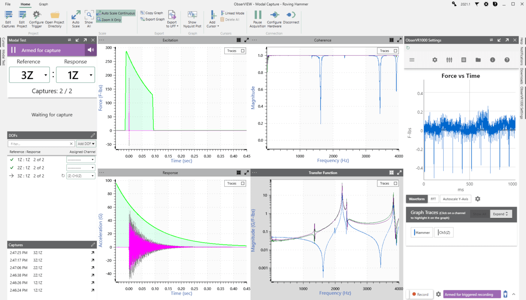
Modal testing software in ObserVIEW.
In the process of data acquisition, an engineer may seek to assess the stability of the closed-loop system. The system’s transfer function displayed as a Nyquist plot can be used to determine this stability.
Modal Data and the Transfer Function
After modal data are acquired, an engineer converts the structure’s response from the time domain to the frequency domain using a Fourier transform. From there, modal software calculates an experimental transfer function (also known as frequency response function). The transfer function provides information about parameters such as modal damping and natural frequencies. The dominant natural frequencies determine the individual modes of the structure.
The transfer function is calculated from excitation and the corresponding response. For a linear and time-invariant system, it describes the ratio of the two signals over a defined frequency range.
The frequency response is complex with real and imaginary parts. Therefore, the transfer function may be normalized by its amplitude response (magnitude) and phase response.
Nyquist Plot for Frequency Response Analysis
Engineers can validate the transfer function between excitation and response with a coherence plot. Coherence is used as a measure of confidence that a peak in the transfer function is a resonant frequency of the device under test and not a spike due to measurement noise.
In the ObserVIEW Modal Testing software, the user can also add a Nyquist plot to view transfer function data as a scatter plot. The Nyquist plot is often used to assess the stability of a system with feedback.
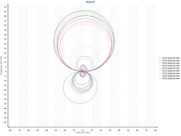
Nyquist plot for experimental data.
The Nyquist plot represents the vector response of a feedback system in the complex plane. The transfer function’s real components are plotted on the x-axis and its imaginary components are plotted on the y-axis for frequencies from – ∞ to + ∞. Frequency is the implicit variable, meaning that each frequency value is a point on the diagram. The plot can also be described using polar coordinates to display the relationship between feedback and gain.
Information Derived from the Nyquist Plot
Frequency response analysis is used to determine the stability and performance of a control system. To analyze a Nyquist plot, engineers apply the Nyquist stability criterion.
The Nyquist stability criterion is a stability test for linear, time-invariant systems and is performed in the frequency domain. It applies the principle of argument to an open-loop transfer function to derive information about the stability of the closed-loop system’s transfer function.
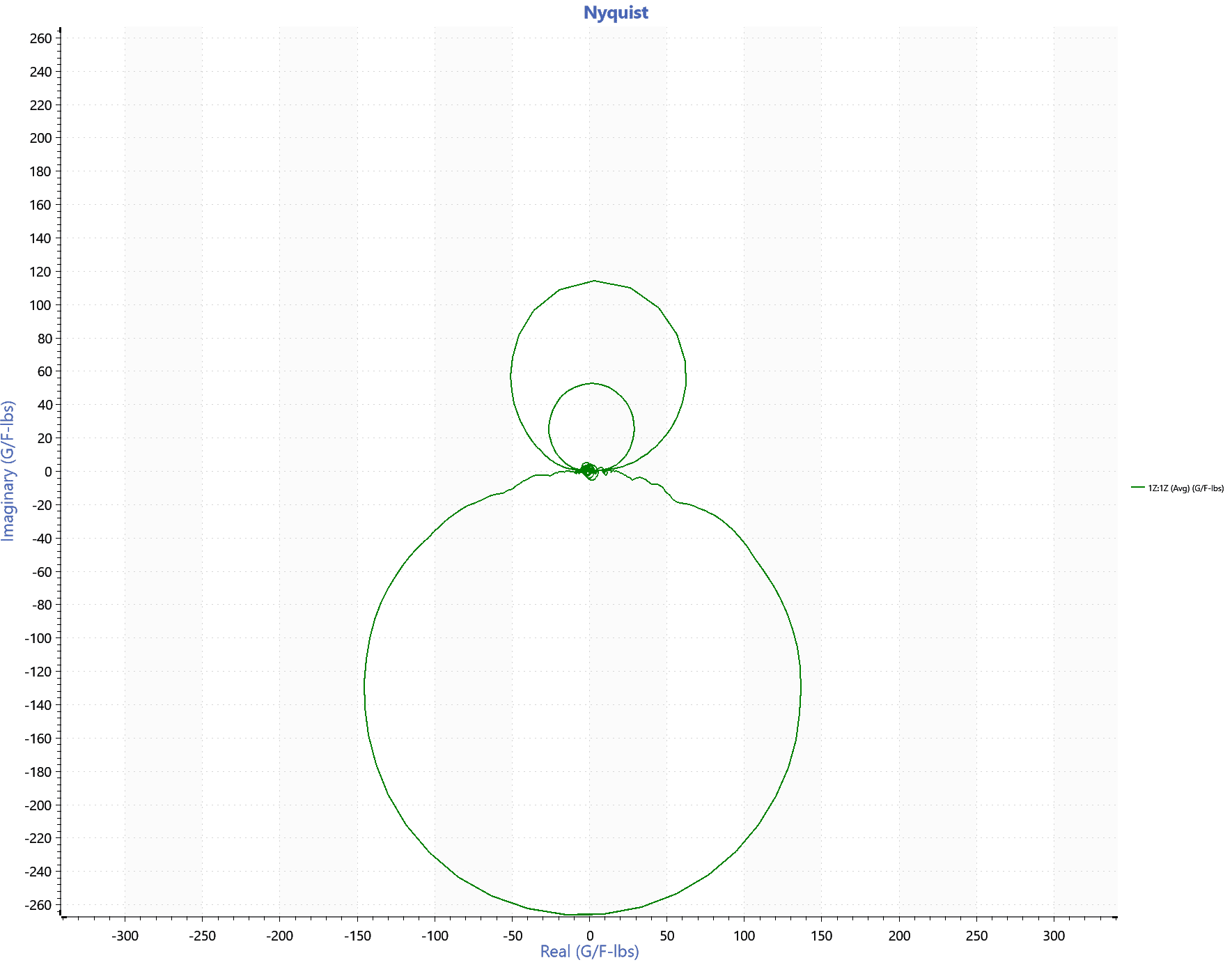
Nyquist plot for a single peak resonance.
The engineer breaks down the Nyquist plot’s data into its real and imaginary traces versus frequency. Then, they break down each lobe into its frequency range subset: 100Hz-200Hz = 1st circle, 500-800Hz = 2nd circle, etc. From there, they can analyze the relative size and direction of the lobe with respect to these components and determine the system’s stability using the criterion.
An engineer can also calculate the phase and gain stability margins from Nyquist plot data, which denote the degree of relative stability.
Modal Testing in ObserVIEW
In ObserVIEW, the user can employ the Modal Testing software to collect a structure’s response to a transient event. The software calculates an average response for each hit location and generates a smooth transfer function (FRF). From there, the collection of FRFs can be exported to a modal analysis software such as MEscope.