Vibration data are recorded as a function of time, meaning the change in some value, such as acceleration, over time. After recording, it is often advantageous to transform the data into a different domain for another perspective. Patterns not readily apparent in the time domain may be visible in others, giving engineers a clearer understanding of their product’s vibrational behavior.
Article Overview
- Overview of Fourier analysis
- Explanation of the fast Fourier transform (FFT) and its purpose
- Efficiencies and limitations of FFT
- FFT in ObserVIEW software for vibration analysis
- FFT parameters: analysis lines, window functions, and averaging
Fast Fourier Transform
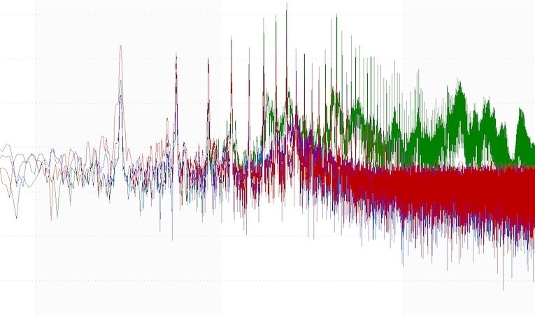
FFT of four channels (inputs).
Vibration test engineers often analyze vibration as a function of frequency. The fast Fourier transform (FFT) is a computational tool that transforms time-domain data into the frequency domain by deconstructing the signal into its individual parts: sine and cosine waves. This computation allows engineers to observe the signal’s frequency components rather than the sum of those components.
The FFT helps engineers determine the excitation frequencies in a complex signal and their amplitude. It also highlights changes in frequency and amplitude and harmonic excitation in the selected frequency range.
For a complex signal, the FFT can help to answer:
- What frequencies are being excited?
- What is the amplitude at each frequency?
- What changes throughout the waveform?
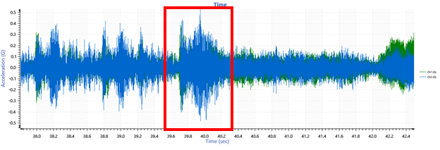
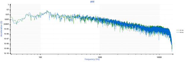
A segment of time-domain data projected onto the frequency domain.
Simplified Explanation of Fourier Analysis
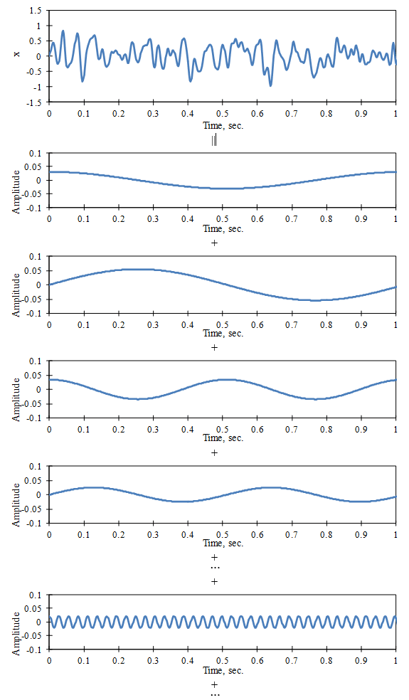
Figure 1. Fourier series construction of a time signal.
Fourier analysis works on the principle that a periodic signal can be represented as a sum of a series of sine and cosine waves. It states that the signal can be separated (analyzed) into a spectrum of discrete frequencies deriving from this series (Figure 1).
The Fourier transform takes apart time domain data using projections. It digitizes the signal, x, into a sequence of N numbers (xn, n = 1 to N). Each sample is a point with a time interval of Δt between them (Figure 2).
The computation calculates the frequency spectra for each sample, including the coefficients (amplitude and phase) that approximate the original signal when combined. Then, it combines the spectra. The resulting set of components is the Fourier transform of x(t).
For a more comprehensive explanation of Fourier analysis, visit the following VRU lessons:
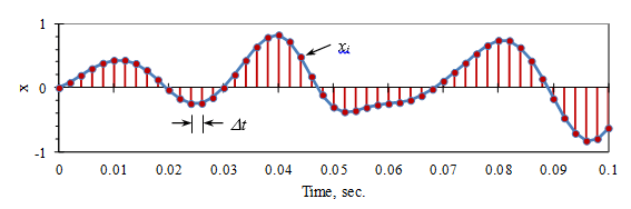
Figure 2. Digitization of a time signal.
The FFT Speeds Things Up
The discrete-time Fourier transform (DTFT) projects a time data sequence of N length onto sinusoids at N frequencies. The FFT performs the same mathematical operation as the DTFT with computational efficiency. Its algorithm uses a sequence of N digital samples where N is a power of 2 (2, 4, 8, 16, 32, etc.).
For example, if a data sequence has a length N=1,024, a DTFT operation would require about N2=1,048,576 operations, whereas the FFT would require about Nlog2(N) = 10,240 operations (about one-tenth as many).
However, this efficiency creates a constraint—the FFT requires the length N to be a power of 2. As such, all analysis line values must also be a power of 2.
FFT Analysis in ObserVIEW
FFT analysis in the ObserVIEW software is an efficient method of data analysis: no code required. The software responds to any change to the settings with a fast and automatic recalculation of the computed parameters. The software can perform the calculation on live data streaming from Live Analyzer or an imported file.
Features of ObserVIEW’s FFT analysis include:
- Up to 1,048,576 analysis lines (user-defined)
- Industry-standard window functions with comprehensive support for the selection process
- Standard, harmonic, and RMS cursor types and more
- Quick reporting features, including copy-paste functionality
- Live computation of data with Live Analyzer
- AVD conversion (acceleration, velocity, displacement)
FFT Parameters
To add a new FFT graph in ObserVIEW, select the Add Graph dropdown button in the main ribbon and select the FFT option. The user-defined settings include analysis lines, window function, and data bias range.
Analysis Lines
The sample rate and analysis lines determine the frame length of an FFT. Fewer lines will result in a shorter frame of time data, and more lines will result in a longer frame.
The length of each frame required to generate an FFT is (analysis lines *2)/sample rate. For pure FFT analysis, the frequency resolution is (sample rate/2)/analysis lines. If the FFT resolution is known, the test engineer can also use 1/FFT resolution to equate the time duration of each FFT frame.
Increasing the number of analysis lines increases the FFT frequency resolution, which is useful when analyzing low-frequency content. Increasing this parameter also results in a higher resolution of the resulting analysis plot. However, higher lines increase the computational burden, and the increased analysis time can result in a slower response to change.
Window Function
The FFT calculation interprets the two endpoints of a time waveform as though they were connected—i.e., they have the same value at each end of a time interval. However, random signals are rarely equal at each end of the time interval. This assumption creates discontinuities in the time domain and results in unwanted noise in the frequency spectrum.
Window functions are added to the signal-processing algorithm to address these discontinuities. ObserVIEW includes the industry-standard window functions including Blackman, Hamming, and Hanning. The user should select the function that best fits the application or the purpose of the analysis. Here are a few tips when selecting a window function:
- Select Blackman, Hamming, or Hanning for general vibration analysis
- Select Rectangular for periodic signals that are shorter than the window length
- Flat Top provides very accurate amplitude measurements, but the user sacrifices frequency accuracy for better amplitude accuracy
- Select Exponential for impact testing, burst random shock, and shock analysis
The ObserVIEW Help file also includes a comprehensive table of window functions for assistance with selection.
FFT Averaging
The FFT computation relies on averaging to combine the samples’ frequency spectra. Linear averaging weighs the data over the time range equally. This approach is reasonable for analyzing the true data of a time frame but does not necessarily reflect the variation of real-world vibration and can flatten peaks that are potentially damaging. Exponential averaging is a moving average that puts more weight on recent data. As such, exponential averaging is favored when analyzing long or non-stationary signals.
Download ObserVIEW
The FFT is the foundation of vibration analysis, offering a computationally efficient method to separate time histories into their frequency components. By understanding its limitations, engineers can apply corrective techniques like windowing, averaging, and analysis line selection to improve data quality. Implemented in tools such as ObserVIEW, FFT enables identification of excitation frequencies, harmonic content, and spectral variations, supporting accurate diagnostics and test development.
Download the free demo of ObserVIEW today and begin analyzing and editing waveforms straight away. Interested in learning more? Visit the software page.