Abstract
Test standards often include a random vibration test to validate a device under test’s (DUT) reliability. Random tests produce a power spectral density (PSD) that identifies resonances across a frequency spectrum and shows if they are within a defined tolerance.
Aerospace test laboratories often test high-value equipment at extremely high levels of random vibration for a brief period. These short-duration, high-amplitude tests are representative of launch and take-off events. The lab’s goal is a realistic test that will identify reliability issues but will not damage the equipment. Ideally, aerospace test engineers want to see a smooth control trace on the PSD that stays within an established tolerance range.
However, does the PSD graph show what is really happening on the shaker table? When it comes to short-duration random tests that are common for expensive launch systems and complex payloads, the answer is not always yes.
Random vibration tests typically have tight tolerances (±1.5dB), so the statistics of averaging fast Fourier transform (FFT) power values make it nearly impossible for all lines to be within tolerance in a short timeframe. In the past, the industry has used unreliable methods to address this issue. In response, Vibration Research developed Instant Degrees of Freedom® (iDOF®): a statistically valid way of generating a smooth PSD during a short-duration random vibration test.
The Estimation Error Problem
The underlying issue with short-duration random vibration testing is the process of PSD estimation. There are two sources of error in a PSD: control and estimation. Control error refers to the discrepancy between the actual PSD of the data and the demand. Estimation error refers to the discrepancy between the signal’s estimated PSD and actual PSD.
Control software generates a PSD by separating time-domain data into a series of frames, calculating the FFT for each frame, and then averaging the power values of the FFTs. The inherent nature of randomness means there is statistical variance in the PSD, which creates estimation error. This error is reduced as more data frames are captured and contribute to the calculation. However, this process takes time, which is something engineers do not have in a short-duration random vibration test.
One approach to avoiding an initially jagged, high-variance display plot is to suppress the PSD display until traces are sufficiently averaged. While this blank display method hides unpleasant early randomness, it also hides events on a shaker early in a test, which can include out-of-tolerance conditions. This situation is clearly dangerous.
Low-level Data Multiplication
Data multiplication is a more common but equally dangerous approach to achieving an attractive PSD for short-duration random vibration tests. It starts the test at a low level. As the test ramps up, it multiplies the low-level data by a scaling factor and presents it as full-level data.
Data multiplication is based on the false assumption that a DUT’s mechanical behavior at the high level mimics the low-level behavior. The mechanical world is not linear. Resonances typically shift in both frequency and amplitude when signal levels change. Data multiplication masks changes occurring at the product resonances, so the test engineer is unaware of potentially damaging vibration energy levels. Multiplying low-level data is inaccurate and misleading.
To illustrate, the white PSD trace in Figure 1 was generated by a test controller at a low-level early stage, while the blue trace comes from an independent signal analyzer. Both traces show essentially the same behavior.
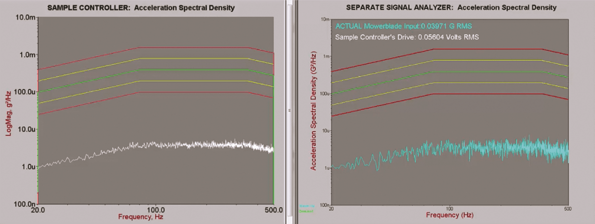
Figure 1. Comparison of a sample controller’s acceleration spectral density to that of a separate signal analyzer. The spectras show essentially the same behavior.
The white PSD trace in Figure 2 is a full-level test generated from data multiplication, while the blue comes from an independent signal analyzer. In this case, the graphs are drastically different. The data multiplication graph does not include the resonant peaks, including some that are well beyond abort limits. An engineer viewing the white PSD cannot see what is happening during the test and has the false impression that it is within tolerance.
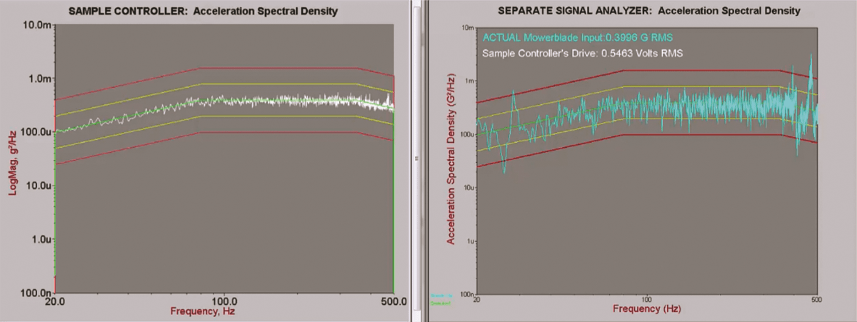
Figure 2. Comparison of a sample controller’s acceleration spectral density to that of a separate signal analyzer. The latter shows the resonant peaks, including some that are well beyond abort limits.
This lack of test level visibility can result in under-testing, meaning the DUT could pass the test but fail during field use, or over-testing, which can damage the DUT. Over-testing error is especially significant if it results in avoidable damage to unique or expensive components or payloads.
Accuracy by Resetting the Average
PSD averaging should be restarted (or reset) with every change in level to accurately display what is happening in the non-linear world. All PSD data are discarded, and the averaging starts over from the beginning.
The advantage of this approach is that it displays the true activity on the shaker. A disadvantage is the time required for averaging a sufficient number of frames. If the trace was within a 1.5dB tolerance at a low level, it would take some time to get back within that tolerance. If your test requires all lines of resolution to be within ±1.5dB, this method will not work.
Note that high PSD estimation variance during the start of a test or a change in level does not mean there is something wrong with the PSD estimation method. Volatility is a natural and expected characteristic of a random signal. The variance is only reduced as more frames of similar data are calculated and averaged into the PSD.
iDOF
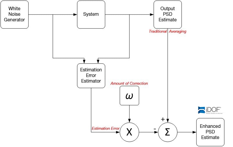 Fortunately, there is a statistically valid way to create an accurate PSD quickly. The variance in random tests is based on Chi-squared distribution. The variance can be calculated and removed from the PSD plot using this statistical understanding (essentially removing the estimation error). (See sidebar: The Statistical Nature of a PSD.) This approach delivers a smooth but accurate PSD, preserving control error so the engineer can view the DUT’s behavior accurately.
iDOF is an optional module in the VibrationVIEW software suite. It uses an advanced algorithm to deliver accurate, low-variance PSD estimates during random vibration testing, calculating its estimates much more quickly than traditional averaging. iDOF removes the estimation error while displaying the control error, which is the true difference between the signal’s PSD and the demand PSD.
With iDOF, control error is visible much sooner than traditional averaging. For example, the iDOF algorithm can process 10 frames of data to produce a PSD estimate comparable to traditional averaging with 100 frames. This speed enables fast detection of changing responses such as shifting resonances (e.g., due to a product beginning to fatigue) without long averaging times, a critical capability for short-duration random vibration tests.
iDOF does not touch the control itself, i.e., it does not affect the signal sent from the controller to the system. iDOF calculations are applied to the estimation of the signal and clarify the estimation of the signal’s PSD. Hence, the control trace more clearly displays the true control signal with less raggedness. After a change in level, iDOF quickly reduces the variance of the PSD estimate without using the low-level data or some other trick. iDOF quickly exposes any lines truly out of tolerance without masking resonances and without requiring the time necessary for traditional averaging.
Figure 4 shows the PSD from a signal analyzer using traditional averaging for a test at full level, while Figure 5 shows the PSD using iDOF at full level. The iDOF PSD preserves and displays the resonances and vibrations experienced by the DUT while significantly reducing the raggedness of the plot. The estimation error has been confidently removed while actual vibrations and deviations from demand due to control are clearly displayed.
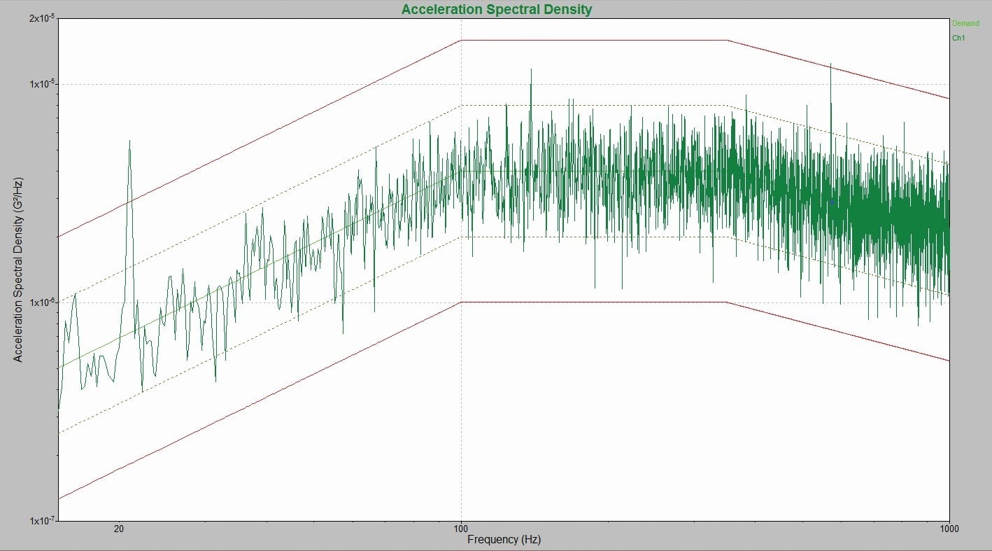
Figure 4: PSD generated by a separate signal analyzer.
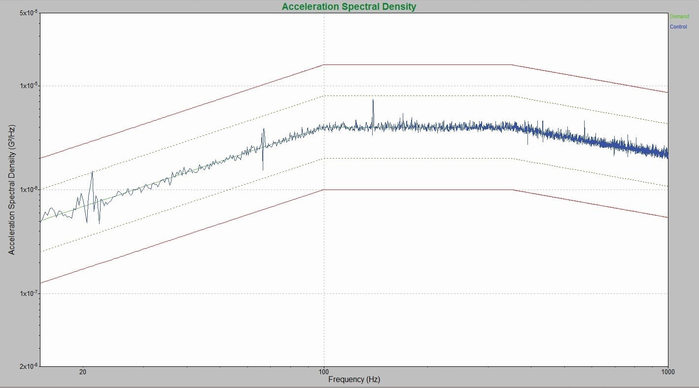
Figure 5: PSD generated using iDOF, with resonances clearly visible.
SUMMARY
Aerospace engineers often run random vibration tests on valuable equipment that must be completed within a brief timeframe. Creating a clear PSD that accurately reflects the test results is difficult because of the time constraint and the statistical nature of PSD calculation. Two common methods that attempt to address this challenge are blank display and low-level data multiplication, but both hide the true test response of a DUT.
After a change in level, iDOF promptly reduces the variance of the PSD estimate and exposes any lines truly out of tolerance without masking resonances. Using iDOF, a test engineer can verify that the control PSD is maintained within tolerance throughout the test and make an informed decision on how a test is affecting the DUT. Most importantly, the engineer can stop a test before the energy from a vibration resonance inflicts damage on an expensive, hard-to-replace DUT.
Sidebar
The Statistical Nature of a PSD
The PSD of a Gaussian random waveform is computed using an FFT. The FFT is a linear transform and it is given a Gaussian input. As a result, the output of the FFT at each frequency line is a complex number, with a Gaussian real part and a Gaussian imaginary part. These are squared and added together to get the magnitude, so the square magnitude of the FFT output is a Chi-squared distributed random variable with 2 degrees of freedom (DOF). To compute an averaged, random PSD, F frames of time data are measured, an FFT for each frame is calculated, and the square magnitudes are averaged together. As a result, the averaged PSD of a Gaussian waveform is a Chi-squared-distributed random variable with 2F DOF.