Developing a Weibull Success-run Sampling Plan

Vibration Research (VR) has provided resources on gathering quality vibration data, correlating it to real-world service life, and using it to develop a vibration test profile with the fatigue damage spectrum (FDS) analysis tools in the VR software. Now, we are taking it one step further by introducing vibration sampling plans and why you need them to ensure product robustness.

In this paper, we define vibration sampling plans, describe the underlying math of the Weibull success-run formula, and demonstrate how to apply it to a vibration test. Doing so will provide realistic insight into whether a product is ready for commercial release.

If you prefer a video format, watch the following webinar.

Success-run Test

Vibration sampling plans state how many repetitions of a vibration test profile—which represents one product service life—must be repeated for a given number of test samples to demonstrate a particular reliability level and confidence level if there are zero failures during the test duration. They typically apply to product validation at the process confirmation stage; however, engineers can use them earlier in product development to aid with reliability growth modeling or as part of a product screening after the start of production.

Testing multiple product samples to failure with a field-correlated test profile is the best way to predict reliability. However, this approach is not always practical due to time and/or lab equipment considerations. Sampling plans demonstrate reliability by testing a pre-defined number of product samples for a set duration with no failures. This approach is called a “success-run” test.

Setting Up for a Sampling Plan

Quality data are essential to developing a vibration sampling plan. Ideally, the engineer would measure the data from the product during a field application. However, this approach may not be practical due to unavailable prototypes, lack of suitable data acquisition hardware and measurement knowledge, or an inaccessible representative environment to record data. The next best option is surrogate data from a similar application, a past event, an industry standard, or an online source. The ObserVR1000 is a portable data acquisition system from VR that engineers can use to gather data in the field and laboratory.

Engineers process the recorded data into a field-correlated vibration test profile with the correct frequency content, amplitudes, kurtosis, and duration. The resulting test profile should represent equivalent vibration exposure to the product’s service life, ideally as defined in its technical specifications. Engineers can use VR’s Fatigue Damage Spectrum (FDS) software to generate a representative test profile.

Then, the engineer must run the test profile in the lab using an appropriately sized shaker, representative fixturing, and optimal control parameters.

Samples on Test

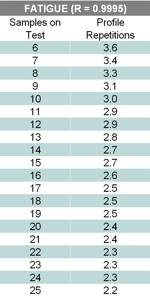
Figure 1. Example sampling plan.

Finally, the engineer can develop an appropriate sampling plan based on Design Failure Mode and Effect Analysis (DFMEA) results that identify the principal vibration-induced failure modes. Figure 1 is an example for fatigue with R99.95C50: 99.95% reliability with 50% confidence. This sampling plan is for illustration; results will differ depending on the product, its intended service life, reliability requirements, and the engineer’s failure mode of interest.

This example has at least six samples on the test. While this number is not always practical depending on the product’s cost and size, at least six samples are generally necessary to gather useful statistics from the results. Attention must be paid to a product’s “bathtub curve” to ensure that, on the low end, the engineer is not testing for so long that the materials wear out rather than failing as expected in the field.

Failure Modes

Different failure modes will be associated with different sampling plans. A vibration test may have multiple sampling plans, starting with the most likely failure mode and increasing/decreasing the test repetitions as needed for that failure mode or others under consideration.

For example, let’s say a test is designed specifically for a solder failure, but a different failure occurs. The engineer can apply an appropriate iteration of the sampling plan to determine if the product has already achieved the reliability requirement with that failure mode, considering the sample size and repetitions for the different failure mode.

Test duration, product hardware numbers, and lab equipment use are well-defined for success-run vibration tests. As such, sampling plans enable optimal use of available resources to minimize test time and cost. They are nearly essential when supplying an OEM on time with parts that satisfy all performance, safety, and reliability requirements.

Sampling plans are essential to the product development lifecycle process.

Static and Dynamic Testing

Conventional engineering thought, often taught in schools, is that a designed-in factor of safety is a good measure of robustness against failure. This thought is true for essentially static situations with few parts, known loads, and materials that have well-known S-N curves. The safety factor is single-valued, theoretical yet practical, and highly deterministic.

For these situations, the factor of safety concept as defined by material ultimate strength or yield strength divided by a known stress level is probably satisfactory.

(1) $\begin{equation*} \text{Factor of safety}=\frac{\text{strength}}{\text{stress}} \end{equation*}$

However, a deterministic approach to predicting failure is insufficient for engineers who work on components or systems with many materials, numerous interfaces, and highly variable cycle-loading environments. Accelerated vibration testing for real-world use is widely variable and stochastic. A different approach is necessary to predict product reliability.

Mathematically, reliability, R(x), can be expressed as the convolution of the stress and strength distributions. The convolution of two functions, f(x) and g(x), is defined as the integral (f∗g)(x).

(2) $\begin{equation*} R(x)=\int^{\infty}_{-\infty}f(t)g(x-t)dt \end{equation*}$

It is a sum of the overlaps of one function and all the shifted versions of the other. When stress exceeds strength, a failure will occur.

Stress-strength Interference

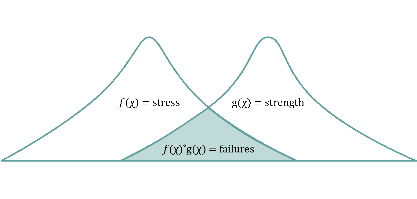
We refer to this convolution as “stress-strength interference.” The stress arises from use in the customer environment, and strength is the design’s resistance to a particular failure mode, such as fatigue or wear, due to materials used, manufacturing variation, inherent defects, etc.

Stress, f(x), and strength, g(x), are distributions; when convolved, they produce a representative distribution of failures as a function of time, miles, cycles, or whatever unit represents use.

Stress f(x) = f(customer use, environment)
Strength g(x) = f(materials, manufacturing variation, defects, etc.)
Integral of f(x)*g(x) = convolution of stress and strength distributions

As mentioned previously, reliability can be expressed mathematically as the convolution of the stress and strength distributions. We need to identify the statistical properties of the distributions to perform the convolution.

Weibull Distribution

First, an overview of common statistics is necessary. Although engineers can use various distributions for this process, the Weibull distribution has such a plasticity that it covers an array of circumstances.

The Weibull distribution is a special case of exponential distribution and helps to model time, distance, cycles, etc., to failure. We use it to model both the stress and strength distributions. For a two-parameter Weibull distribution, the probability density function (PDF) is:

(3) $\begin{equation*} f(x)=\frac{\beta}{\theta}\left(\frac{x}{\theta}\right)^{\beta-1}e^{-(\frac{x}{\theta})^{\beta}} \end{equation*}$

Where:

theta ( $\theta$ ) is a scale parameter; often referred to as the characteristic life and the time at which 63.2% of the parts have failed
beta ( $\beta$ ) is the shape parameter; often referred to as the Weibull slope and directly related to failure mode
f(t)≥0, $\beta$ ≥0, and $\theta$ ≥0

Engineers can linearize the Weibull distribution for readability/understandability. Linearization produces a common form of the Weibull graph with unreliability on the vertical axis (1-failure rate expressed as a percent) and time to failure on the horizontal axis (or miles, cycles, etc.).

Figure 2 shows the Weibull PDFs for the three linearized versions in Figure 3. We can readily see the adaptability of the Weibull distribution. A Weibull slope of 3 is approximately normal, while a Weibull slope of 1 is exponential. Slopes less than one generally have a decreasing failure rate as a function of time (or miles, cycles, etc.), whereas Weibull slopes greater than 1 have an increasing failure rate.

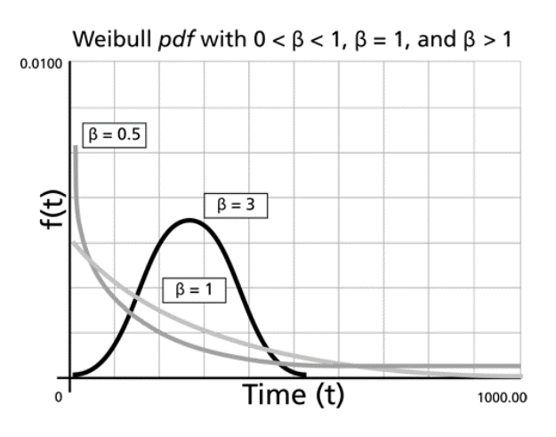
A Weibull PDF. The graph has three lines with slopes of 0.5, 1, and 3.

Figure 2. Weibull probability density functions (PDF). Image credit: Kate Racaza via reliawiki.com.

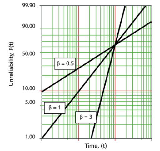
A linearized version of a Weibull PDF. The graph has three lines with slopes of 0.5, 1, and 3.

Figure 3. Linearized versions of Figure 2 traces. Image credit: Nicolette Young via reliawiki.com.

Sampling Plan

Now, let’s work through an example of how to develop a sampling plan. For this example, let’s imagine that we have relative damage numbers that represent 20 customers over the service life of our product. We want to design a success-run sampling plan for a vibration test that demonstrates R99.95C50: 99.95% reliability with 50% confidence. A 99.95% confidence means we are willing to accept five failures out of 10,000.

There are four steps to the process.

Step 1

In step 1, we estimate the Weibull parameters for the stress distribution using customer data.

First, we list the 20 customers and their relative damage numbers (Figure 4). Then, we rank the numbers from smallest to largest. Their respective median ranks are calculated using the given median rank formula:

(4) $\begin{equation*} \text{median rank}=\frac{j_i-0.3}{n+0.4} \end{equation*}$

Where:

$j_i$ is the rank
n is the number of samples

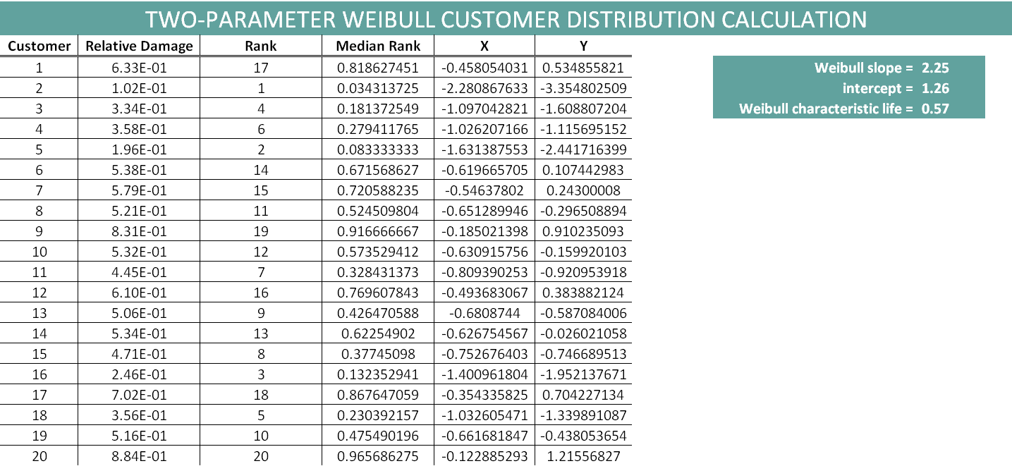
A six-column table with customer data for calculating distribution. The columns represent relative damage, rank, median rank, x, and y.

Figure 4. Customer data for calculating distribution.

Next, we make a linearized Weibull plot by graphing the natural log of the customer relative damage numbers against the natural log of the natural log of 1 minus the median rank (Figure 5). We can fit this data to a least squares regression best-fit line and get the Weibull slope ( $\beta$ ). Using the intercept value, we can estimate the characteristic life ( $\theta$ ) as e to the minus (intercept over Weibull slope). The characteristic life is the time (or miles, cycles, etc.) at which 63.2% of the parts have failed.

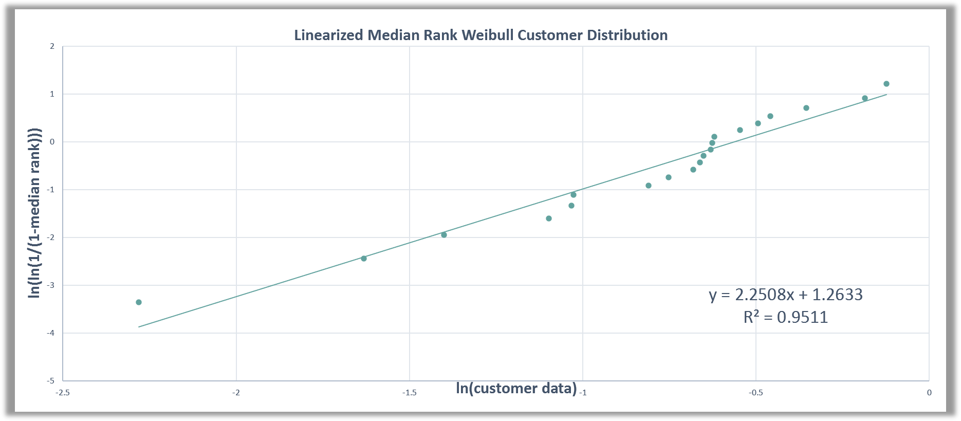
A linearized median rank weibull customer distribution with the natural log of the customer relative damage numbers on the x axis and the natural log of the natural log of 1 minus the median rank on the y axis.

Figure 5. Linearized Weibull plot of customer data.

Often, measured customer data are unavailable. In that case, engineers can obtain pseudo-customer data from proving ground measurements, surrogate data from similar applications, virtually synthesized data, or other sources. Engineers can use this data in a randomized fashion to develop a distribution of customer use.

Now, we have estimated Weibull parameters for the stress distribution. We still need Weibull parameters for the strength distribution to perform our stress-strength convolution.

Steps 2 and 3

In steps 2 and 3, we will determine the Weibull parameters for the strength distribution. We need to assume a Weibull slope ( $\beta$ ) for the failure mode of interest. For this example, we will use $\beta$ = 3 as a generic representation of a fatigue failure mode.

Then, we must use a convolution routine made using R, Python, Excel, or another software to back-calculate a value for strength characteristic life ( $\theta$ ) such that the stress and strength distributions overlap to equal the desired failure rate (Figure 6). The desired failure rate equals 1 minus the desired reliability; for our example, it is 0.0005.

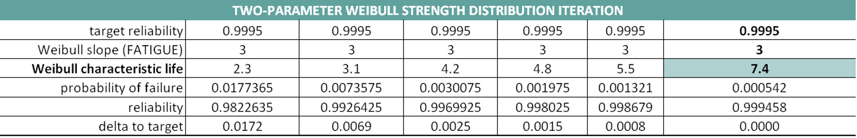
A six-row weibull convolution routine to back-calculate a value for strength characteristic life. The rows include target reliability, Weibull slope, Weibull characteristic life, probability of failure, reliability, and delta to target.

Figure 6. Back-calculating a value for strength characteristic life.

As the table shows, we made several guesses, starting with $\theta$ = 2.3, which was too low. Other guesses were theta values of 3.1, 4.2, 4.8, and 5.5, walking up to the converging value of $\theta$ = 7.4.

We will hold on to this value for step 4, but we must first digress to talk about the “standard” binomial success-run formula, which, in turn, will be used to develop the Weibull success-run formula.

Binomial Probability Distribution

The binomial PDF is given by the formula:

(5) $\begin{equation*} P(x)=\frac{n!}{x!(n-x)!}p^{x}q^{(n-x)} \end{equation*}$

Where:

n is the number of samples on the test
p is the probability of failing
q is the probability of not failing
x is the number of failures

Binomial probability is appropriate when the following conditions are satisfied:

The sample size is fixed
Samples are independent
The only outcomes are a failure or no failure
The probability of failure is constant

These are the conditions for a success-run testing situation.

Note that because the binomial distribution is discrete, we can use a summation to calculate cumulative binomial probability:

(6) $\begin{equation*} P(0\leq x \leq n )=\sum^{n}_{x=0}\frac{n!}{x!(n-x)!}p^{x}q^{(n-x)} \end{equation*}$

This summation tells us the probability of zero to all of our parts failing during the test if we know, in general, the probability of a part failing. We assume this to be our failure rate or 1 minus the desired reliability.

Confidence Level

For our purposes, we will define confidence level as C=n-x: the number of samples on the test that did not fail. In our example, we will set C equal to 50%, or 0.50, which is common as it equalizes the producer’s risk (overestimating reliability) and the consumer’s risk (underestimating reliability).

The complement of C is the number of samples on the test that did fail, which is equal to 1-C.

If we let p=1-R be the probability of a sample failing, and let q be the complement of p, which is the probability of no samples failing, then q=1-(1-R)=R.

Substituting these values into the binomial probability distribution, we can express the cumulative probability as:

(7) $\begin{equation*} 1-C=\sum^{n}_{x=0}\frac{n!}{x!(n-x)!}(1-R)^{x}R^{(n-x)} \end{equation*}$

Binomial Success-run Formula

Success-run testing means that zero failures are allowed, so we set x equal to zero in our binomial probability distribution and find:

(8) $\begin{equation*} 1-C=\sum^{n}_{x=0}\frac{n!}{0!(n-0)!}(1-R)^{0}R^{(n-0)} \end{equation*}$

(9) $\begin{equation*} 1-C=\sum^{n}_{x=0}\frac{n!}{n!}(1)R^{n} \end{equation*}$

So,

(10) $\begin{equation*} 1-C=R^{n} \end{equation*}$

(11) $\begin{equation*} \ln(1-C)=n\ln R \end{equation*}$

(12) $\begin{equation*} n=\frac{\ln(1-C)}{\ln R} \end{equation*}$

This is the success-run formula. It looks like we are good to go; however, there is a problem.

The binomial success-run formula assumes we are testing each part to only one service life. That means for R99.95C50, we must test 1,386 product samples without any failures.

(13) $\begin{equation*} n=\frac{\ln(1-C)}{\ln R}=\frac{\ln(1-0.50)}{\ln(0.9995)}=1386 \end{equation*}$

This scenario is unrealistic, so let’s revisit our previous Weibull math and see if we can combine these distributions to reach a more achievable number of test parts and test time.

Weibull Revisited

Recall that the PDF for the two-parameter Weibull distribution gives the probability of a failure as a function of time (or miles, cycles, etc.):

(14) $\begin{equation*} f(x)=\frac{\beta}{\theta}\left(\frac{x}{\theta}\right)^{\beta-1}e^{-(\frac{x}{\theta})^{\beta}} \end{equation*}$

Accordingly, the cumulative density function gives the probability of x number of failures over an interval of time (or miles, cycles, etc.). We found it by integrating the Weibull PDF:

(15) $\begin{equation*} \int^{x}_{0}f(x)dx=\int^{x}_{0}\frac{\beta}{\theta}\left(\frac{x}{\theta}\right)^{\beta-1}e^{-(\frac{x}{\theta})^{\beta}}dx=1-e^{-(\frac{x}{\theta})^{\beta}} \end{equation*}$

Finally, the cumulative reliability function is the complement of the cumulative Weibull:

(16) $\begin{equation*} R(x)=1-\left[1-e^{-(\frac{x}{\theta})^{\beta}}\right]=e^{-(\frac{x}{\theta})^{\beta}} \end{equation*}$

Recalling that 1-C=R^n from our derivation of the binomial success-run formula, we can rearrange terms to get: R=(1-C)^(1/n).

If we equate this expression with the Weibull cumulative reliability function that we derived earlier, we can solve for x:

(17) $\begin{equation*} e^{-(\frac{x}{\theta})^{\beta}}=(1-C)^{\frac{1}{n}} \end{equation*}$

(18) $\begin{equation*} -\left(\frac{x}{\theta}\right)^{\beta}=\ln(1-C)^{\frac{1}{n}} \end{equation*}$

(19) $\begin{equation*} -\left(\frac{x}{\theta}\right)^{\beta}=\frac{\ln(1-C)}{n} \end{equation*}$

(20) $\begin{equation*} \left(\frac{x}{\theta}\right)^{\beta}=\frac{-\ln(1-C)}{n} \end{equation*}$

(21) $\begin{equation*} \frac{x}{\theta}=\left[\frac{-\ln(1-C)}{n}\right]^{\frac{1}{\beta}} \end{equation*}$

(22) $\begin{equation*} x=\theta\left[\frac{-\ln(1-C)}{n}\right]^{\frac{1}{\beta}} \end{equation*}$

Now, we have a Weibull version of the success-run formula, where n is the number of samples on the test that must pass without failing, and x is the number of profile repetitions needed to demonstrate the desired reliability level.

We can use this formula to optimize test time and lab resources, and it gives us statistical confidence in the meaning of the test with respect to reliability.

Let’s see how it works out for our example.

The following are Weibull success-run sampling plans for three situations:

R99.95C50 for fatigue
R99.50C50 for fatigue
R99.95C50 for wear

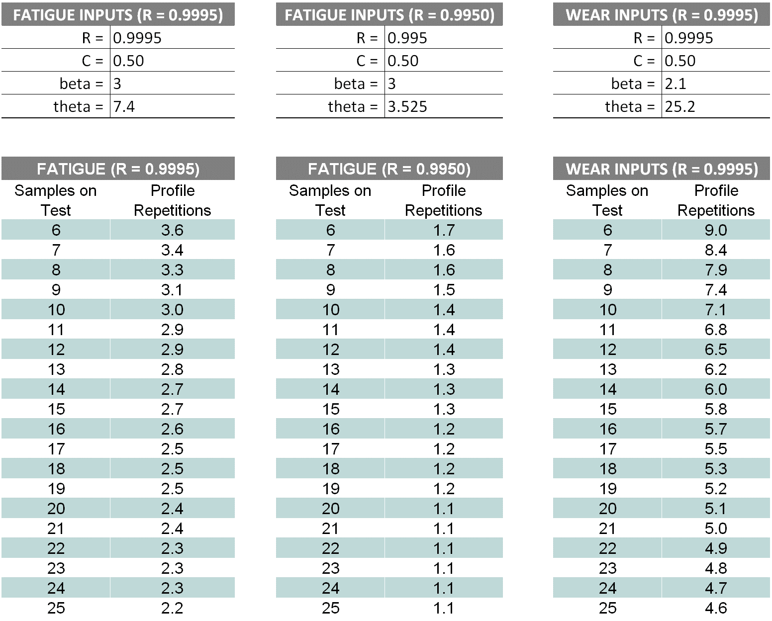
Figure 7. Three examples of Weibull success-run sampling plans.

For the wear failure mode, we assumed a Weibull slope equal to 2 for our strength distribution and subsequent back calculation for wear characteristic life.

The higher reliability requires longer testing; going from R99.95C50 to R99.90C50 for fatigue on six samples goes from 3.6 profile repetitions to 1.7.

Likewise, reducing the Weibull slope as we did for wear significantly increases the test length for a given reliability.

Conclusion

Identifying failure modes is an effective use of product development resources. For vibration testing, this means having quality data that is measured and analyzed correctly to correlate an accelerated test or virtual twin to a known amount of severe customer use. With the right tools and know-how, acquiring good data and using it to arrive at a vibration test profile with the appropriate frequency content, amplitude, and duration is readily achievable. VR hardware and software give test engineers the confidence that their test profiles deliver field-representative results.

Developing a sampling plan and using it to optimize test hardware and lab equipment scheduling can save time and money while instilling confidence that your product will exceed your customer’s reliability expectations. Appropriate use of the success-run formula to make a vibration sampling plan confirms that your product is ready to release to commerce.

Developing a Weibull Success-run Sampling Plan

Experiments and Papers

Author Tom Achatz

Success-run Test

Setting Up for a Sampling Plan

Samples on Test

Failure Modes

Static and Dynamic Testing

Stress-strength Interference

Weibull Distribution

Sampling Plan

Step 1

Steps 2 and 3

Binomial Probability Distribution

Confidence Level

Binomial Success-run Formula

Weibull Revisited

Conclusion

How Can We Help You?