This paper originally appeared in Test Engineering & Management Magazine, June/July 2004.
In vibration testing, there are quite a few test types to which you can expose your product. The primary choices are sine, random, classical shock, transient shock, field-recorded time history, sine-on-random, random-on-random, and sine-and-random-on-random. Our customers often request advice on which test type to run and, in particular, how to choose between the two most common test types: sine and random. They want to know which test, sine or random, most quickly pinpoints flaws in their product. If they can only run one of the two tests, which should it be?
Recently, I received an even more specific request from a customer. They presented data from a sine test and a random test and wanted to know: given both a sine test and a random test, how he could determine which is the most severe? Let’s take a look at the two tests and decide how to answer his question.
The Question
How would the following specifications compare in amplitude/severity?
Sine Test (Figure 1)
- 3.5G at 5Hz to 50Hz
- 1.5G at 50Hz to 300Hz
- Limit vibration to 0.4in double amplitude
- Test all axes at the same level
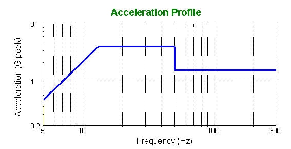
Figure 1: Sample sine test profile.
Random (Figure 2)
- 0.01500 G2/Hz from 10Hz to 0.01500G2/Hz at 40Hz
- 0.01500 G2/Hz at 40Hz to 0.00015G2/Hz at 500Hz
- Results in 1.05GRMS
- Test all axes at the same level
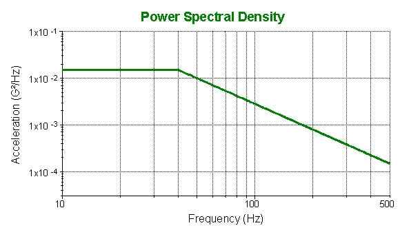
Figure 2: Sample random test profile.
The Response
This is a valid and interesting question. Why? Because the answer is not obvious. The sine vibration is measured in G peak (Gpk), while the random vibration is measured as GRMS, with the peak G levels typically left to a statistical assumption. A quick calculation tells us that the random test, which can have peak values up to 4 or even 5 times the RMS level, will apply 4 x 1.05 GRMS, or 4.20Gpk to our product. Since the sine test is only 3.5 Gpk, we would expect the random test to be more damaging, right?
Analysis
Looking for support from some equations, let’s make some reasonable assumptions: 1) failures due to vibration are caused at the peak G level seen by the product, 2) most products have resonances at one or more frequencies, and 3) at these resonances the vibration levels applied to the product are amplified by the Q factor of the resonance. Following this train of logic, we conclude that the failures will occur when the vibration is at one of the resonant frequencies. Now when we use a sine vibration, the full vibration levels are concentrated at the resonant frequency, and the vibration levels are simply amplified by the amplification factor Q.
(1) Aproduct,sine = Q x Acontrol,sine
When we use a random vibration, it is not so simple because not all of the vibration is amplified by the resonance. Let’s further assume the resonance has a Q factor of 5 or more. In that case, the resonance will act as an amplifying band-pass filter with amplification equal to Q, and a bandwidth equal to Df, where
(2) Q = fn / Δf
fn = resonant frequency
Δf = half-power bandwidth of the resonance
It will also be helpful to refer to the following relationship, which tells us that, for a given RMS level, the PSD level is inversely proportional to the full bandwidth of the random spectrum. In more general terms, a more concentrated random vibration will have a higher PSD value.
(3) PSDcontrol = Acontrol,rms2 / ΔF *
ΔF = full bandwidth of the random PSD
*equation (3) applies to flat spectrum only
A random test is defined in terms of a PSD, which is an amplitude-squared measure. So, at the resonant frequency, the PSD levels of the product will be amplified by Q2. Since the resonance acts as an amplifying band-pass filter, we can approximate the vibration levels at the product by looking at just the energy at the resonant frequency that passes through and is amplified by the resonance (again assuming the random waveform has up to 4 sigma peaks):
(4) Aproduct,peak = 4 x Aproduct,rms
= 4 x [ PSDproduct x Δf ]1/2
= 4 x [ Q2 x PSDcontrol x Δf ]1/2
= 4 x [ PSDcontrol x Q x fn ]1/2
From equation (4) we note three features of the peak amplitude for a random test:
- It is proportional to only the square root of Q. As a result, a high-Q resonance will result in a more severe test in sine than it will in random if all other parameters are equal.
- It is proportional to the square root of the resonant frequency, fn, so the higher the resonant frequency, the higher the peak values in the output.
- Referring back to equation (3), we also note that the more concentrated the random vibration is, the higher the peak vibration levels will be.
Now we can also compare the peak vibration levels on the product for both Sine and Random tests by comparing equations (1) and (4) with Aproduct,sine = Aproduct,peak,random.
(5) Acontrol,sine = Aproduct,sine / Q
= Aproduct,peak,random / Q
= 4 x [ fn x PSDcontrol / Q ]1/2
Equation (5) allows a direct comparison of a random test with a sine test, for a given value for the Q factor. We plotted our two test specifications in Figure 3, where we see that the sine equivalent to our random test is actually a much lower test level than our sine test. Only in the case of resonance at 50Hz, where the sine test steps down in amplitude, with Q=5 does the random test level even come close to the sine test level. So the equations are telling us that the sine test will be more severe than the random test.
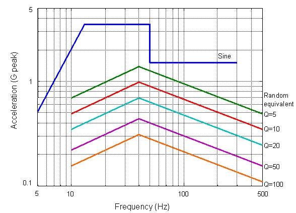
Figure 3: Comparison of the Sine equivalents to the Random profile, with various Q. For higher Q, the Sine equivalent to the Random profile has a lower amplitude.
Application
At the time the customer asked his question, I was at Sperry Marine in Charlottesville Virginia, setting up for some equipment installation training. This was a great time to demonstrate and test for the differences. As a single test is worth a thousand opinions, we set up to run both the random test and the sine test on a slip plate (Figure 9). The slip plate had two elements mounted on it, each with different resonant frequencies. The elements were aluminum masses attached by threaded rods of different lengths and thicknesses, with accelerometers mounted on the mass at the top of each rod connected to channels 4 and 6.
What we needed to do for the comparison was run the tests, and then look at the G levels seen. We knew they would be 3.5Gpk for the sine test at the control point, and, making a 4-sigma peak assumption, we expected to find 4.2Gpk at the control point for the random test also. The two plots in Figures 4 and 5 show the controlled test along with the response data for the two vertical rods with masses attached.
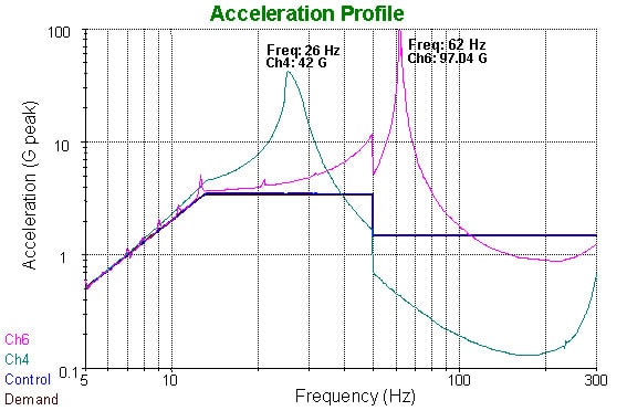
Figure 4: Sine test results.
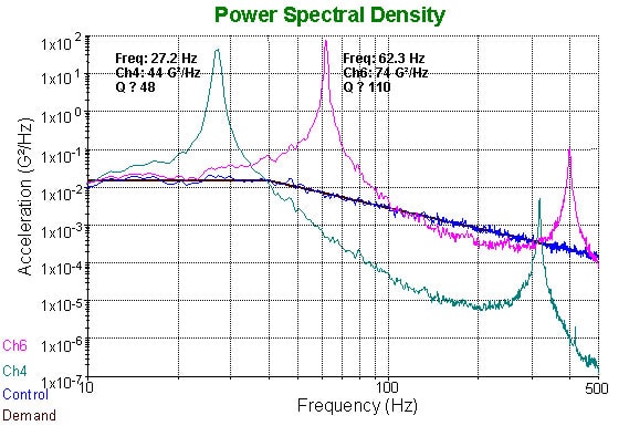
Figure 5: Random test results.
While running the tests, we also simultaneously streamed the accelerometer data to the hard disk drive for later analysis. This allowed us to be able to make a direct comparison of the peak G levels for each of the tests. As expected, at the control point, the peak G levels for the Sine test were 3.5Gpk and 1.5Gpk. The random test levels at the control point were 1.05GRMS, as expected, and 4.8Gpk, which is a little bit higher than the 4-sigma peaks we predicted, but not unusual for a Gaussian random vibration (Figure 6).
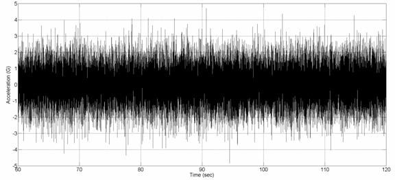
Figure 6: At the control point, the Random test vibration levels showed a 4.8Gpk.
Now, as we were running the test, we observed the resonant elements mounted to the slip table going berserk. This also showed up on the controller plots (Figures 4 and 5), which showed much larger accelerations on channels 4 and 6 than measured at the control point. What could be going on here? Recall from equations (1) and (4) above, that when we have resonances in the product, they will amplify the vibration levels. The accelerometers monitoring our two resonant elements show the resonance frequencies are 27Hz and 62Hz, right in the middle of our test range.
Let us examine the time data for those accelerometers, which we had conveniently streamed to the hard disk drive, and see what is happening at the resonant elements. This may shed more light on the test equivalences. First looking at the frequency response for the Ch4 accelerometer (Figure 5), we estimate a Q factor of 48 and a resonant frequency of 27Hz. However, we note that the bandwidth, Δf = fn / Q = 0.6Hz, which is less than the frequency resolution of the PSD plot (using 800 lines). This is a good indication that the Q factor estimated from this PSD will be underestimated. Since we had recorded the time waveforms to disk, we are able to load these waveforms into Matlab™ and use high-resolution spectral post-processing (13,000 lines) to zoom in on the peaks. With this more accurate estimate, we find the Q level to be 140. Computing using equation (4), we expect a peak level of 4 x [ 0.015 x 140 x 27 ]1/2, or 30Gpk. Figure 7 shows the actual acceleration levels on Ch4, where we find the peak G level was 28G.
Next looking at the frequency response for the Ch6 accelerometer (Figure 5) we estimate a Q factor of 110 and a resonant frequency of 62Hz. Again we find the bandwidth, 0.6Hz, to be less than the frequency resolution of the PSD plot, so we need to post-process this recorded waveform to obtain a more accurate estimate of the Q factor. Using 13,000 lines of resolution we estimate the Q factor to be 200. Computing using equation (4), we expect to see peak levels of 4 x [ 0.00673 x 200 x 62 ]1/2, or 37Gpk. Figure 8 shows the actual acceleration levels on Ch6, where we find the peak G level was 42G.
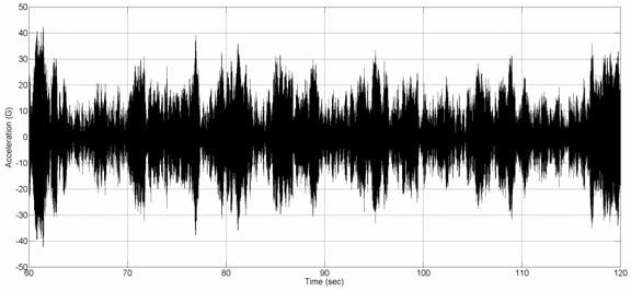
Figure 7: On Ch4, the Random test vibration levels showed a 28Gpk.

Figure 8: On Ch6, the Random test vibration levels showed a 42Gpk.
Observations
Let’s make a table of the results, so we can get the whole picture:
| Q | Sine (G peak) |
Random (GRMS) |
Random (G peak) |
Predicted (Eqn. 4) (G peak) |
|
| Control point | – | 3.5G | 1.05G | 4.8G | 4.2G |
| Ch4 (27Hz resonance) | 140 | 42G | 8.35G | 28G | 30G |
| Ch6 (62Hz resonance) | 200 | 97G | 10.9G | 42G | 37 |
From these results, we find that at the control point, the random test has higher peak G levels than the sine test. This would lead us to believe that the random test was a more severe test. However, at the resonant points, the sine test has higher peak G levels than the random test. From the product’s perspective, the sine test was the more severe test.
You may also notice that the sine resonance peak values were not as high as would be predicted by the Q factor. By reviewing the recorded time data for Ch4 we are able to determine that, at the 27Hz resonance, the sine sweep passed through the resonance too quickly to fully excite the resonance. Repeating the test using a slower sweep rate or a resonance search-and-dwell feature would allow us to more accurately find the resonance frequency and Q factor. From this, we can conclude that for high Q values, to get the full Q amplification effects of a sine test, you must either sweep slowly or do a resonance dwell at each resonance.
By examining the recorded data for Ch6, we are also able to determine that at the 62Hz resonance, the acceleration levels were so high that they exceeded the accelerometer’s measurement capacity, and therefore the measured waveform was saturated well below the actual acceleration levels. This is an important point because quite often accelerometers are sized based on the test profile’s acceleration level, while the resonances may see 10x or 100x the profile acceleration level. Repeating the test using a higher capacity accelerometer is required to accurately measure the acceleration levels at that resonance.
The actual random peak values are a little different from the predicted values, but this is to be expected due to the random nature of the waveform. Each random test you run will be different from any other random test, so the peak values will vary from test to test, and even over different time intervals within a single test.
Conclusion
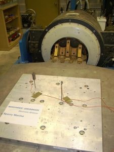
Figure 9: Test setup in the lab at Sperry Marine, Charlottesville, Virginia.
The relative severity of a sine test and a random test will vary depending on your product’s resonant frequencies and Qs. In general, when sine and random tests have the same peak vibration levels at the control point, the product will see higher vibration levels with a sine test than with a random test due to the resonances in the product. Equation (5) gives you a way to convert a random PSD into an approximately equivalent sine peak acceleration, as long as you know the resonant frequencies and Q factors of the product.
However, you must also consider that a sine test only excites a single product resonance at a time, so a sine test will not test the interaction between two resonances in your product. Since a random test excites the full frequency range all at the same time, it can be used to find problems resulting from the interaction between two resonances.