Abstract
This technical note defines the function of the m and Q values when creating a fatigue damage spectrum (FDS) in the VibrationVIEW or ObserVIEW software programs and accelerating an FDS-correlated random test profile.
Question
- What is the purpose of the m and Q values in reference to the fatigue damage spectrum?
- What values of m and Q can I use as a starting point for the test development of a mixed composition component?
- How can I determine more specific m and Q values?
Answer
The FDS uses one or multiple time-history files to create an accelerated random test profile that is the damage equivalent to the relative environment. The m value and the resonance factor (Q) are used to calculate the fatigue damage values that make up the FDS.
Q Value
The Q value determines the spread of damage throughout the frequency spectrum of the resulting PSD test profile. A low Q value spreads damage amongst neighboring frequencies, and a high Q concentrates the damage. A higher Q value uses narrower filters resulting in sharper peaks, while a lower Q results in a wider filter and a smoother spectrum with less detail.
If the Q value of the product is unknown, a good starting value is 10. A Q of 10 outputs an FDS—and thus, a PSD—with a reasonable filtering and frequency response.
To determine a more specific value for Q, perform a simple sine sweep through the operating range of the product to find the primary resonance. The Q value for the FDS should be the Q of the primary resonance.
m Value
The m value is an exponent in the FDS equation, so it plays a larger role than Q, which is a divisor in the equation (Henderson & Piersol, 1995). MIL-STD-810H provides some direction for defining an initial m value when the S-N curve or m value of a product is unknown.
“The value of ‘m’ is generally some proportion of the negative reciprocal of the slope of the S-N curve, known as the fatigue strength exponent and designated as ‘-1/b.’ Typical values of ‘m’ are 80 percent of ‘-1/b’ for random waveshapes, and 60 percent of ‘-1/b’ for sinusoidal waveshapes. Historically, a value of m = 7.5 has been used for random environments, but values between 5 and 8 are commonly used. A value of 6 is commonly used for sinusoidal environments.”
The m value affects the processes of FDS generation and test compression differently. A number between 5 and 8 is a good starting point, but the engineer should consider this difference when selecting a value. The engineer must also account for the type of random data imported. Typically, real-world data are non-Gaussian. If the input waveform is Gaussian (kurtosis = 3), the resulting PSD is the same regardless of the m and Q values.
The following sections describe the effects of the m value on FDS generation and test time compression with non-Gaussian data.
FDS Generation with Non-Gaussian Data
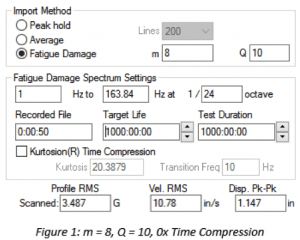
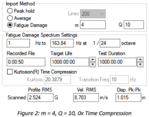
For non-Gaussian data, a higher m puts more weight on peak values than a lower m, meaning the high kurtosis peaks play a greater factor in FDS generation. The resulting test will have a higher acceleration, velocity, and displacement, making it more conservative than the imported time-history file. Figure 1 and Figure 2 show the resulting PSD profile values for the same time-history file with different m values.
| m value | RMS (G) | Vel. RMS (in/s) | Disp. pk-pk (in) |
| 8 | 3.487 | 10.78 | 1.147 |
| 4 | 2.524 | 8.703 | 1.015 |
Table 1. Comparison of acceleration, velocity, and displacement for different m values.
Test Time Compression with Non-Gaussian Data
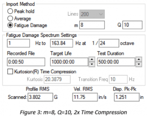
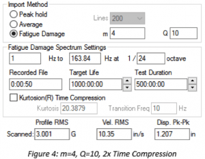
The m value has the opposite effect for test time compression with a non-Gaussian input waveform. With a higher m, an increase in time reduction has less of an effect on the increase in PSD amplitude. Compare Figure 3 and Figure 4. When m = 8 at a 2x time compression, there is an approximate 10% increase in the profile gRMS. When m=4 at a 2x time compression, the increase is 20%. For time compression, failure is more likely when using a lower m value.
Determining a Specific m Value
The accuracy of the m value can significantly improve the accuracy of FDS generation. The process to determine the m value is more involved than that of determining Q. To accurately determine m, an S-N graph (stress to number of cycles) is required (Wöhler, 1870).
One method of producing the S-N graph is to repeatedly test a product to failure at varying gRMS levels and record the time required to reach failure. With enough failure runs recorded, it is possible to back-calculate a strong approximation of the S-N curve by:
- Plotting the data points on a log-log graph
- Plotting the power-law model of the data
The slope of the power-law model is equal to b. From b, it is possible to calculate the value of m.
(1) 
SF is based on the recommendations of MIL-STD-810H:
“The value of ‘m’ is strongly influenced by the material S-N curve, but fatigue life is also influenced by the surface finish, the treatment, the effect of mean stress correction, the contributions of elastic and plastic strain, the waveshape of the strain time history, etc. Therefore, the value of ‘m’ is generally some proportion of the negative reciprocal of the slope of the S-N curve, known as the fatigue strength exponent and designated as ‘-1/b.’ Typical values of ‘m’ are 80 percent of ‘-1/b’ for random waveshapes, and 60 percent of ‘-1/b’ for sinusoidal waveshapes.”
Vibration Research has an m calculation tool that plots the gRMS vs. time to failure data, determines the slope of the S-N curve, and calculates the m based on the input data.
Adding Kurtosis
Adding kurtosis to the PSD reduces the effect of m due to the decrease in overall gRMS caused by the addition of higher kurtosis peaks. Although the generated FDS accounts for the damaging kurtosis peaks in the original time-history file, adding kurtosis to the resulting PSD can be helpful. Adding kurtosis lowers the test’s overall gRMS requirement while maintaining a damage profile equivalent to the imported time-history file. This action can be particularly beneficial when an amplifier can handle the peaks but is unable to maintain the continuous demand of the PSD.
Conclusion
Overall, if the m and Q values for a product are unknown, an initial recommended starting point would be:
- m=6 or 8 (sinusoidal or random)
- Q=10
These values create a conservative FDS with reasonable filtering and frequency resolution. As more data are accumulated, these values can be adjusted to accurately estimate a product’s m and Q values, even if it is a mixed composition component.