This paper originally appeared in Sound & Vibration Magazine, August 2007, pp. 12-20.
Dynamic range is one of the fundamental metrics describing the capability of a shaker controller. We all know that dynamic range describes the span of small-to-large acceleration amplitude that can be properly controlled during a test. Since modern controllers are digital instruments, we also know the dynamic range to be “six times the number of bits in the analog/digital converter.” But what do we really know? Let’s examine the dynamic range of a vibration controller more scientifically.
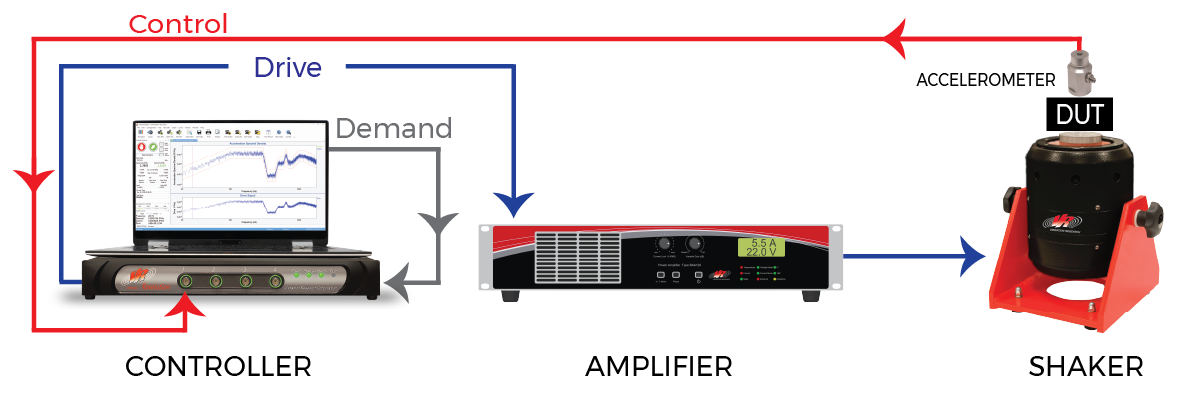
Figure 1. A vibration controller generates a Drive signal that causes the measured Control acceleration to closely match a prescribed Demand.
As shown in Figure 1, a controller forms a loop around the shaker and device under test (DUT) by providing an analog signal to the power amplifier driving the shaker’s armature (or control valve) voice coil. This signal is called the Drive and the controller forms it by comparing the (analog) Control acceleration measured on the shaker table (or upon the DUT) with the desired Demand reference. The control algorithms seek to systematically minimize the difference between the Control and Demand signals by adjusting the shape and amplitude of the Drive signal.
It is clear from Figure 1 that the available dynamic range of a test is limited not only by the controller dynamic range but also by the characteristics of the power amplifier, shaker, control-point accelerometer, test object, and all the mounting hardware and methods employed. It is also clear that the controller’s role involves measuring the Control signal, performing calculations and processes upon this measurement, and generating the Drive signal. The amplitude depth of each of these three processes affects the available test dynamic range.
The shaker and its amplifier must be powerful enough to drive the DUT and fixturing to the required force and motion levels of the test. The shaker’s suspension must be sufficiently linear to accurately reproduce the low amplitude details of the Demand and the amplifier’s noise floor must be low enough not to mask these features. The accelerometer and its signal conditioning must have an adequate dynamic range to follow the Control motion with fidelity and this range must be properly matched to the acceleration span of the test. When all of these conditions are met, the controller becomes the limiting factor in the loop’s performance. Hence, it is important to have a controller with as much dynamic range as possible.
You can never have too much dynamic range in any piece of test equipment. Physical realities of a test always stack up unfavorably to consume every ounce of available dynamic range a system can muster. It is also important that you understand the dynamic range of your equipment so that you can accurately predict test system performance analytically. This avoids employing time and laboratory assets on a “wing and a prayer” basis, always a costly operating philosophy.
dB(SNR): What Dynamic Range Really Says
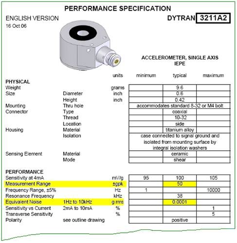
Figure 2. Typical specifications of a modern accelerometer (courtesy Dytran Instruments).
Dynamic range is the ratio of the largest and smallest signals that can be simultaneously properly processed by an instrument or system. This ratio is normally expressed in decibels (dB) to compact the range of numbers we need to think about. The largest signal is the full-scale input or output, while the smallest is the noise floor or resolution limit of the process. Thus the dynamic range is really a signal-to-noise ratio (SNR) expressed in dB. Quite often, physics demands that the full-scale and noise-floor specifications be presented in a dimensionally-inconsistent manner. It is common to know the full scale as a peak value and the noise floor as a root-mean-square (RMS) value. Consider the accelerometer specifications shown in Figure 2 as an example.
This 100 mV/g sensor has a measurement range or full-scale of ±50 g and an equivalent noise, or noise floor, of 0.0001 g RMS. The full scale reflects the largest peak acceleration that can be measured without clipping or limiting the output (voltage) signal. In contrast, the sensor’s noise floor is a continuous broadband spectrum. Hence, the minimum resolvable signal is expressed as an RMS value over a specified bandwidth (1 Hz to 10 kHz in this case). Note that this noise-floor likely changes ‘height’ with frequency; if it were flat, it could be expressed as a constant g/√Hz spectral density or g2/Hz power spectral density.
Dynamic range is always expressed as a ratio of consistent numbers. Hence, we will assume the ±50 g full-scale signal to be a sinewave and use its RMS value (0.707*50 gpeak = 35.4 grms) in the dynamic range calculation. This gives us a full scale-to-noise floor ratio of 35.4 divided by 0.0001 or 353,500; converting this number to decibels yields 111 dB (= 20*log10[353,500]). Note that a sinewave is always used for such peak-to-RMS conversion by industry convention. Also, note that the 111 dB dynamic range is for the frequency span of 1 Hz to 10 kHz. If the sensor’s input is confined to a narrower bandwidth, the dynamic range will actually increase, reflecting the integration of the noise floor over a smaller frequency interval. The same characteristic is found in vibration controllers.
Testing Your Controller
To test the dynamic range of a device it is necessary to use a carefully constructed signal which has a peak value just below the maximum level that the device can measure, and also has a small signal that is just above the noise floor. These two signal levels could be at the same frequency and applied sequentially, or else could be two simultaneous signals applied at different frequencies. The dynamic range measurement is the ratio between the largest signal that can be measured, and the smallest that can be measured.
No single test can fully tax and capture all aspects of a controller’s dynamic range. However, the following group of tests collectively documents a particular instrument’s capabilities. Each test has strengths and weaknesses which will be discussed. Some of these tests require external equipment; such tests must be approached with some trepidation. It is all too easy to lay off the frailty of the inexperienced operator or an external instrument on the controller under examination. Digital storage oscilloscopes typically have an 8-bit resolution, and function generators rarely are harmonically pure to -100 dB. Modern vibration controllers are as accurate as most digital signal analyzers and often will be the most accurate function generator and signal analyzer in your lab.
We will use tests that focus on three aspects of the controller: input channels, output channels, and control algorithms. These three aspects will be interdependent, especially the control algorithm tests, which depend on the signals from the input and output channels, and therefore can be no better than either of those. In many cases, both the controller input and output will be used simultaneously.
We will look at two different tests of an input channel, wherein carefully produced external analog signals are applied to the Control input and the controller is used to capture the signal for digital analysis. Then we will examine the dynamic range of the Drive output by having the controller generate a full-scale fixed-frequency sinewave and measure this with an external signal analyzer. Next, we will use a severe Demand spectrum in a bare-wire, or loop-back, test to examine both the Drive and Control signals, simultaneously. Two additional loop-back tests will be discussed, one using swept sine and the other narrow bands of random noise. Finally, we will examine controlling a high-Q active filter acting as a simulation of a structure on a shaker.
Two-Tone Input Test
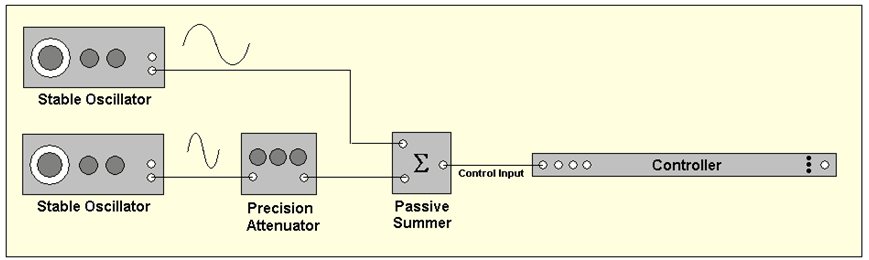
Figure 3. Testing the dynamic range of Control input using the two-tone method.
The two-tone dynamic range of a Control input channel is borrowed from the IEEE recommended practice for testing a time-compression or FFT spectrum analyzer. As shown in Figure 3, an analog signal with two sinewave components is applied. One component is adjusted to be a full-scale input. The second sine, at a different frequency, is attenuated until it is just ‘lost’ in the baseline of a spectrum computed from the sum. The ratio of these components is determined by the setting of a precision attenuator, and this setting is recorded as the dynamic range when the smaller signal is just indistinguishable from the spectral floor.
The test signal required for this test may be generated by a high-performance arbitrary function generator. Alternatively, two high-quality oscillators or sine synthesizers, a precise attenuator, and a precision summing circuit may be used to build the signal. The analog sine sources need to provide an output greater than the full scale of the controller input channel, to allow the use of a passive summing circuit. Using an active summer introduces an external noise floor to the equation and introduces possible signal artifacts including intermodulation products.
The results of this test depend strongly on the block length used for the FFT and the type of window function used. The quantization noise of the primary tone acts as a dither signal, and this allows the measurement of low amplitude signals that could not be measured independently. For example, with a 65,536 sample block length and a Hanning window function, an ideal 14-bit system would show 120 dB with this test. Obviously, this is much greater than the 84 dB SNR one would normally expect from a 14-bit input. For this reason, this test is not a good measure of dynamic range.
Also, note that the frequency peaks due to harmonic distortion will in all likelihood be higher than the lower of the two summed signals. If the two signals being measured are harmonics of each other, then the level of harmonic distortion will be the limiting factor. This is evident in Figure 4, where the harmonics of the primary tone are more prominent than the low-level tone. So, while the noise floor allows for distinguishing some signals 135 dB apart, this test may be more useful as a measure of the amount of harmonic distortion present. What cannot be determined from this test is whether the harmonic distortion is due to the arbitrary function generator or is due to the controller input electronics.
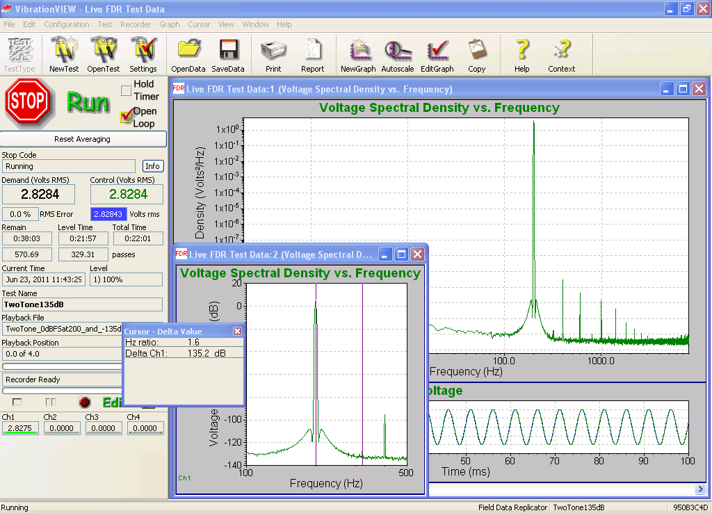
Figure 4. Two-tone test of VR9500 controller indicates 135 dB between full scale and small tone.
Effective Bits Input Test
This is a more recent test method sanctioned by the IEEE for digital recording devices. As shown in Figure 5, a single sinewave is applied to the Control input channel. An untriggered digital recording of the sine is made by the controller input hardware and this data is curve-fitted to yield the four parameters (f, A, B, and C ) of a model of the form: y(t) = A Cos(2 π f n Δt) + B Sin(2π f n Δt) +C, where Δt is the known inter-sample interval and n is the sample count. This parameter identification allows the ‘signal’ to be separated from the noise, permitting the calculation of an SNR. The result is then expressed in terms of effective bits rather than in dB.
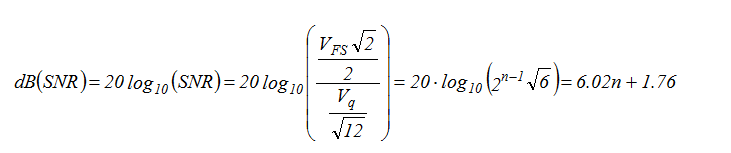
To understand the conversion from dB(SNR) to effective bits, consider the perfect n-bit converter. A perfect n-bit converter exhibits 2n unique output codes uniformly spanning its ±VFS input voltage range. Each “least significant bit” (LSB) change in the output code reflects a change in input voltage by an amount, Vq, termed the quantization voltage, where Vq = VFS / 2n-1. Note that the code representation is exactly correct at only 2n specific voltages; in all other cases, it is in error by as much as ±Vq/2. Hence the converter is said to be precise to ± ½ LSB. As a result, the ideal converter has an RMS noise floor of Vq/√12. When a sine signal of ±VFS peak is applied to the converter, the (RMS) signal/noise ratio is given by:
 (Equation 1)
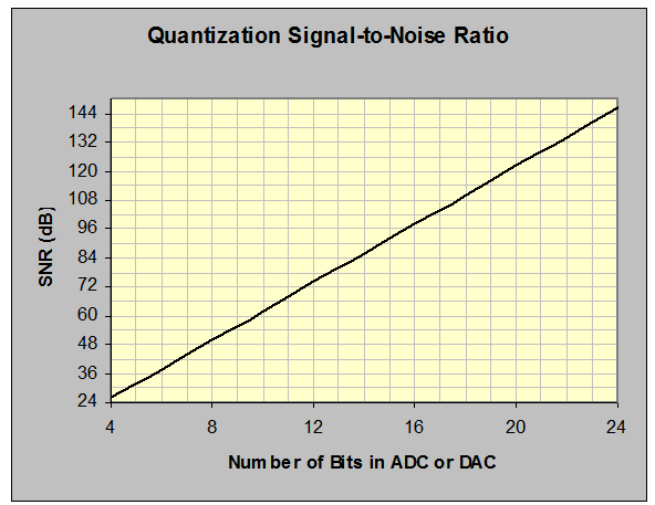
Figure 6. Relationship between effective bits and dynamic range or SNR.
This result is plotted in Figure 6, and we now have a better understanding of the long-accepted 6 dB-per-bit truism! Effective bits compress a large range of numbers into a more comprehensible span, as does a dB calculation. For example, the accelerometer previously discussed has a claimed SNR of 111 dB. Use this number to enter the vertical axis of Figure 6; read the equivalent number of bits (slightly more than 18) from the horizontal axis. Clearly, this sensor would have no problem feeding a 16-bit ADC to full dynamic range capability. It would be a clear choke point in a 24-bit system.
The major advantage of an effective bits test is that it requires no comparative measurements. The frequency of the test sine must be within the selected bandwidth of the controller. Its amplitude must be less than the ±Fs voltage of the input. However, neither the frequency nor the amplitude of the test signal needs to be measured or known. The sine must be stable in frequency and amplitude and pure in the waveform. For this reason, the analog filtered output of a digital synthesizer is the preferred signal source. However, the controller must provide access to the raw waveform data, and a digital curve-fitting algorithm is required to accomplish the test. The IEEE particularly warns against using an FFT as the curve-fitting process and recommends the direct application of least-squares minimization between the model and the acquired samples.
This test was run on a Vibration Research VR9500 controller, using the controller output as a high-quality sine wave synthesizer and the RecorderVIEW feature to record the raw input waveforms to disk. These waveforms were then loaded into MATLAB® and processed with a curve-fitting algorithm. Typical test results for the VR9500 are shown in Figure 7.
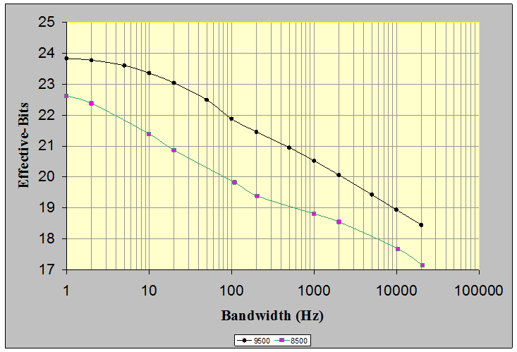
Figure 7. Measured Effective-Bits of the VR9500 and VR8500 Control input channel at various bandwidths.
The four test bandwidths of 20 Hz and less correspond to the selected sine tracking filter bandwidths. The six higher bandwidths show typical broadband results; these include the 200 Hz ASTM transportation test bandwidth, the 2,000 Hz NAVMAT test bandwidth, and the VR9500’s maximum bandwidth. The corresponding dynamic ranges for these bandwidths are shown in Figure 8.
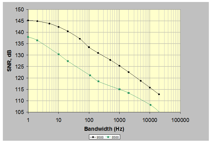
Figure 8. Dynamic range of the VR9500 and VR8500 controller at various bandwidths.
Single-Tone Output Test
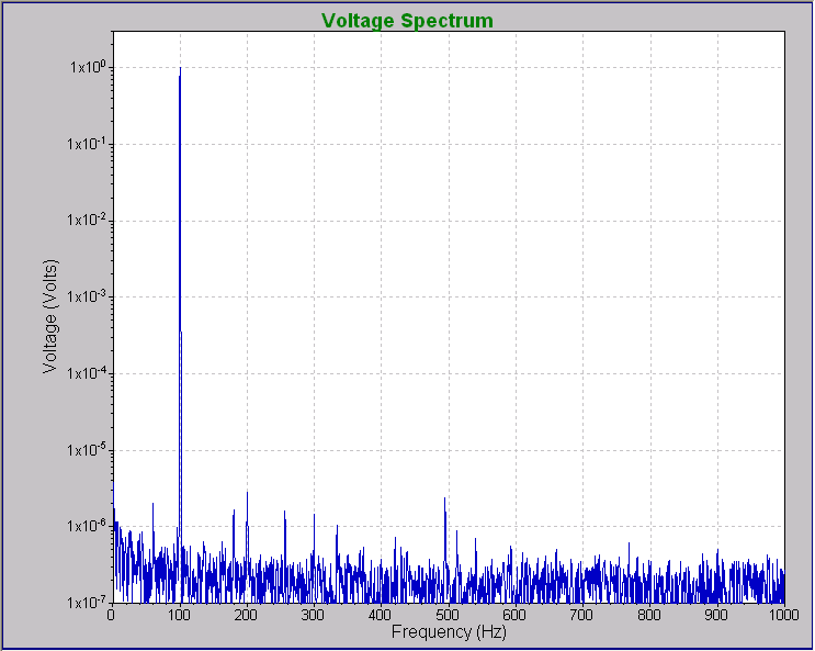
Figure 10. This single-tone test of the VR9500 Drive output shows roughly 110 dB dynamic range.
Figure 10 shows the spectrum of a 1,000 Hz ±2 Volt sine generated by a VR9500 controller output and analyzed using an external FFT analyzer. The background noise is more than 126 dB below the signal, with the highest harmonic peak about 110 dB below the signal.
Loop-back Tests
The drawback of the preceding tests is the requirement for external equipment and/or external mathematical analysis. However, vibration controllers have the ability both to produce output and analyze the input, and both of these functions are used simultaneously while in operation. Therefore it is desirable to apply a test, which uses the controller’s output and input so that both are tested simultaneously, and no additional equipment is required. The results of the test will then reflect the combined dynamic range of both the outputs and inputs. It is also possible to do these same tests with only the output, using an external signal analyzer, or only the input using an external signal synthesizer. This would allow separate results to be stated for both the output and the input, at the expense of requiring additional equipment.
Sine Loop-Back Test
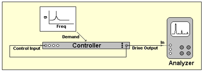
Figure 11. Ramped-sine loop-back test setup.
In this test, the Drive is looped back to the Control input as shown in Figure 11. A swept-sine test is run, with the test specifying a fixed frequency sine with an exponential decrease in amplitude over the duration of the test. The amplitude starts at the full-scale level and then decreases to a level below the anticipated dynamic range of the controller. The Drive and Control are viewed as RMS-versus-time plots with a log amplitude axis. The Transmissibility (RMS-to-RMS ratio) of the Control with respect to the Drive is also displayed.
Both of these traces are clean straight lines within the dynamic range of the controller. The amplitude is at the controller’s full scale on the left side of the display and sweeps down into the noise on the right. In this region, the transmissibility is exactly 1.0 (for 1000 mV/g). At the (right) edge of the dynamic range, where the envelope of the transmissibility spans .707 to 1.41, the signal and noise values are at the same amplitude. The Drive voltage RMS at this point in the test is equal to the instrument’s RMS noise floor within the frequency band passed by the tracking filter. The amplitude of the drive voltage at this point is therefore a measure of the noise floor. The dynamic range of the output and input is the ratio of the maximum voltage (full-scale voltage) to this noise floor measurement.
It is important to note here that the RMS noise floor in this test is the amount of noise measured after the tracking filter. The narrower the tracking filter, the less noise it will pass through. Therefore the sine tracking filter bandwidth is an important parameter in this test, and when using the results of this test to compare controllers, it is important to use the same bandwidth for each controller. Figure 12 illustrates that the VR9500 controller, with a 10 Hz tracking filter bandwidth, shows a dynamic range of more than 130 dB.
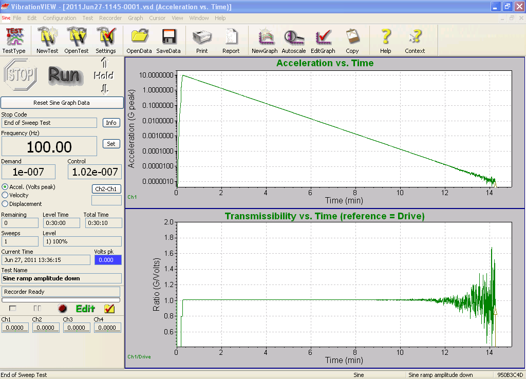
Figure 12. Ramped-sine test of the VR9500 controller indicates about 130 dB input/output dynamic range.
Random Loop-back Test
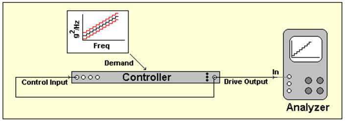
Figure 13. Narrow-band random loop-back test setup.
The controller can be tested in a similar manner using a random test, employing a sequence of stepped demand levels ranging from below the noise floor to the full-scale spectral density as shown in Figure 13. To determine the lower limit the coherence between the Drive and Control is computed. The lower limit is the level prior to the point where the coherence drops below 0.5. The dynamic range measurement is then the ratio of the full-scale density over this lower limit. The full-scale density for this test is determined by the level where the RMS of the highest band nearly makes the signal peaks reach the full-scale voltage. This will happen when √(Densitymax*Bandwidth) = VFS/6 where VFS is the full-scale voltage level, and bandwidth is the frequency width of the steps used. The implication of this is the full-scale spectral density will depend on the bandwidth used in this test, and as a result, the resulting dynamic range measurement will depend on the bandwidth used in the test.
The narrower the bandwidth used in the test, the higher the maximum density level that can be achieved, and therefore the wider the dynamic range value that will be reported. Because of this, when comparing controllers using this test one must be careful to use the same parameters on both controllers.
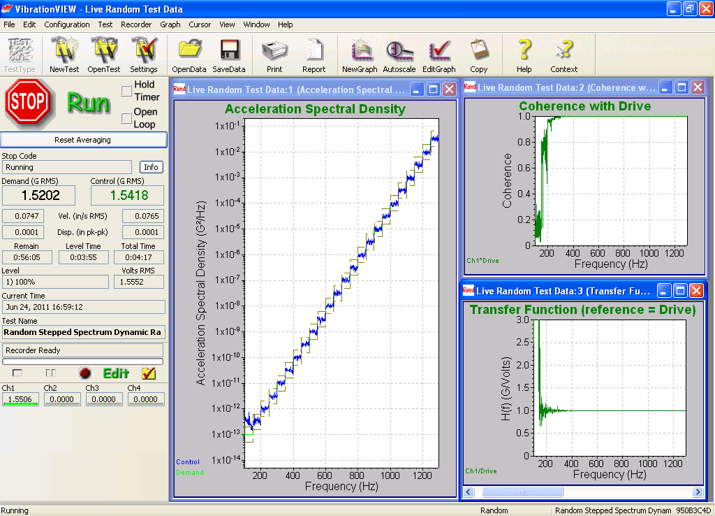
Figure 14. Random test indicates 105 dB of clean dynamic range for the VR9500.
Figure 14 shows a loop-back random test being run on a VR9500 controller. As shown, 24 Demand PSD steps, each 50 Hz wide, span 115 dB. The control appears to be tight from 3.16 x 10⁻² V2/Hz down to 1 x 10-13 V2/Hz, a span of 115 dB.
However, the accompanying coherence and transmissibility plots indicate that the noise floor is closer to 3.16 x 10⁻¹³ V2/Hz for a conservative random dynamic range of 105 dB. Note that the coherence is greater than 0.9 all the way down to –105 dB. It is still about .8 at –110 dB where the transmissibility departs from 1.0.
Note that this test is run with a Demand PSD that has increasing amplitude steps with frequency. This assures that the lowest amplitude steps in the Control signal reflect the instrument’s noise floor rather than harmonic distortion. That is, no step of this signal introduces significant harmonics of itself in other steps.
Input/Output Test Using a Severe Demand
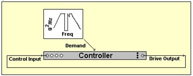
Figure 15. Testing both Drive and Control dynamic range using a severe Demand.
An interesting alternative to the previous tests was developed by the Chinese government around 1988. This test (see Figure 15) is meritorious in that it requires no external equipment; it taxes both the Control input and Drive output simultaneously. It requires the tester to understand nothing beyond the operation of the controller and does not involve curve-fitting or advanced mathematics. In short, it is absolutely elegant in its simplicity.
The key to this efficient evaluation is the frequency span between 350 and 500 Hz, as shown in Figure 15. The Demand spectrum in this region is successively programmed to lower g2/Hz power spectral density levels until the controller fails to conduct the test. The lowest notch level at which control can be achieved determines the control system dynamic range.
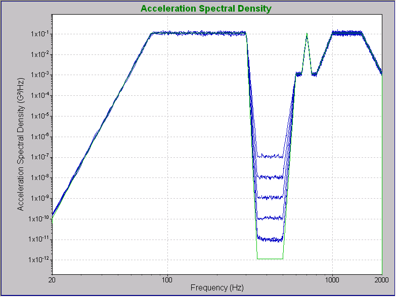
Figure 16. VR9500 performing the Chinese JJG 529-88 challenge test at 60 through 110 dB.
As shown in Figure 16, the VR9500 successfully controlled the notch down to a depth of –100 dB with respect to the highest PSD level. It could not follow the –110 dB demand of the lowest figure. Figure 17 shows the 100 dB test in more detail, including the limits and the Drive signal.
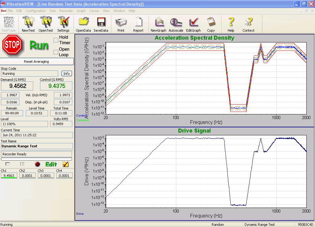
Figure 17. Details of JJG 529-88 operation at 100 dB for VR9500 showing Control with Limits and Drive signal.
Note that the JJG 529-88 test profile is specified in g2/Hz units. Also, recall that to test dynamic range the signals used must be carefully crafted such that the peak levels are just below the maximum value the system is capable of measuring. Therefore the operator must select the mV/g sensitivity of the (non-existent) accelerometer such that the peak levels of the 10 gRMS signal are just below the maximum input voltage of the system, for the input range being tested. This allows this test to be independent of the input range used. For a system with ±10 Volt Control and Drive full-scales, this optimum is about 100 mV/g, which results in voltage levels of 1 VRMS, and 6 VPEAK At this point the achievable depth of the notch will measure the range between the full-scale signal and the noise floor. If the sensitivity is increased above 200 mV/G then the waveform peaks will begin to saturate. This will be evident as a sudden increase in the measured G2/Hz level in the 350-500Hz notch, and will severely impact the test results.
Now if we factor out the sensitivity scale factor and consider the relationship between the maximum V2/Hz level and full-scale input voltage, and also the relationship between the minimum V2/Hz level and the noise floor, we can get some more insight into this test. For the given spectrum, the maximum PSD level is 10-3 times the square of the RMS voltage, VRMS. Assuming a crest factor of 5, the maximum achievable VRMS level will be VFS/5. The minimum achievable V2/Hz level, assuming a flat noise spectrum, will be (Vnoise2)/(2000 Hz), where Vnoise is the RMS noise floor. The expected random dynamic range (RDR) of the JJG 529-88 test will then be the dB ratio of these two power spectral densities.
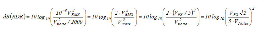 (Equation 2)
This result can be recast in terms of the SNR measured in an effective bits test. VNoise can be recognized as including the quantization noise of an ideal converter and the noise of the supporting signal conditioning. Therefore the RDR can be restated in terms of SNR as follows.
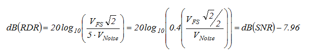 (Equation 3)
This is a very interesting result because it tells us that the best results one could expect from this test will be 8 dB less than the dB(SNR) as measured using a sine tone. This is to be expected because the peaks in a random signal are higher than for a sine signal, so the random full-scale RMS will be lower than the sine full-scale RMS.
To apply these results practically, we refer to Figure 8 and note that for the VR9500 with a 2,000Hz bandwidth, the SNR is 122 dB, so we could reasonably expect a 114 dB result from the JJ 529-88 test. But we only found a result of 100 dB. What accounts for this difference? The answer lies in the high band from 80 to 300Hz. The notch from 350 to 500Hz corresponds to the harmonics of the 80 to 300Hz band. Any harmonic distortion of the 80 to 300Hz band will show up as an increased noise level in the 350 to 500Hz notch. Therefore this test measures dynamic range up to a point (typically to 16 effective bits), but beyond that point, the results are limited by harmonic distortion. Since most current controllers have more than 16 bits of resolution, their results using this test will be limited by the harmonic distortion of the system, and not by the dynamic range.
Random Algorithm and Output Test Using a High-Q Filter to Simulate a Shaker and Structure
There is one valid criticism that can be directed at the JJ 529-88 test: it does not demonstrate control over any sharp resonance peaks and notches that may exist in a structure. Our next test addresses this issue. At least two controller manufacturers have built active challenge filters and issued them to their sales staff for field demonstration purposes. These two designs are remarkably similar; both manufacturers selected similar peak and notch frequencies and amplitudes. The VR9500 was recently tested against the newer of these two challenge filters.
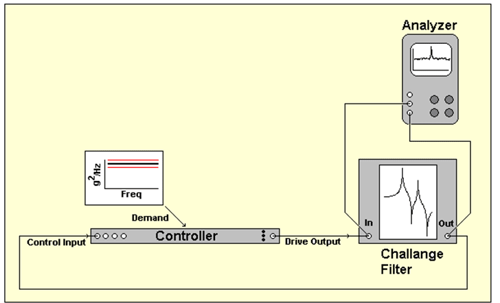
Figure 18. Testing dynamic range by closing the loop around a simulation filter.
In this test, the filter is driven by the Drive signal, and its output is applied to the Control channel as shown in Figure 18. The test Demand is a flat spectrum spanning 20 Hz to 2,000 Hz. Thus, when fully controlled, all of the significant signal dynamics will be reflected by the Drive signal. The implication of this is the test exercises the control algorithm and the output signal, but since the reference spectrum is flat, the input dynamic range is essentially untaxed by this test.
Testing these filters is a challenge until a couple of things are understood. Firstly, the filter uses active electronics with a limited voltage range, The filter becomes wildly non-linear when it is overloaded. Neither design incorporates any form of overload indication, so the experimenter needs to determine the maximum white drive that can be applied without causing the filter to grossly misbehave.
Secondly, the filter’s DC gain of 10 (20 dB) is a bit deceptive. As it would suggest, the RMS output of the filter is greater than the RMS input, when the input frequency is below the frequency of the first peak. However, when a white input is applied to the filter, the output RMS is about 36 dB greater than the input RMS. Then, when the input is properly ‘shaped’ to produce a white filter output, the output RMS is about 23 dB less than the input RMS.
All of this means that the test must be conducted with a properly chosen RMS demand level. The 20 dB DC gain might lead one to think the reference spectrum should be chosen to give 1VRMS. But once the drive signal is properly shaped to make the filter output white, the filter input would be 23 dB higher than 1VRMS, or 14.6VRMS. Clearly, this would overdrive the filter input! The proper choice of the demand level is found by determining the input level that overloads the filter and then setting the reference spectrum to be 23 dB lower than this level. Typically such a filter will work properly up to a 1VRMS input, so setting the reference spectrum to give 68mVRMS would yield the best results.
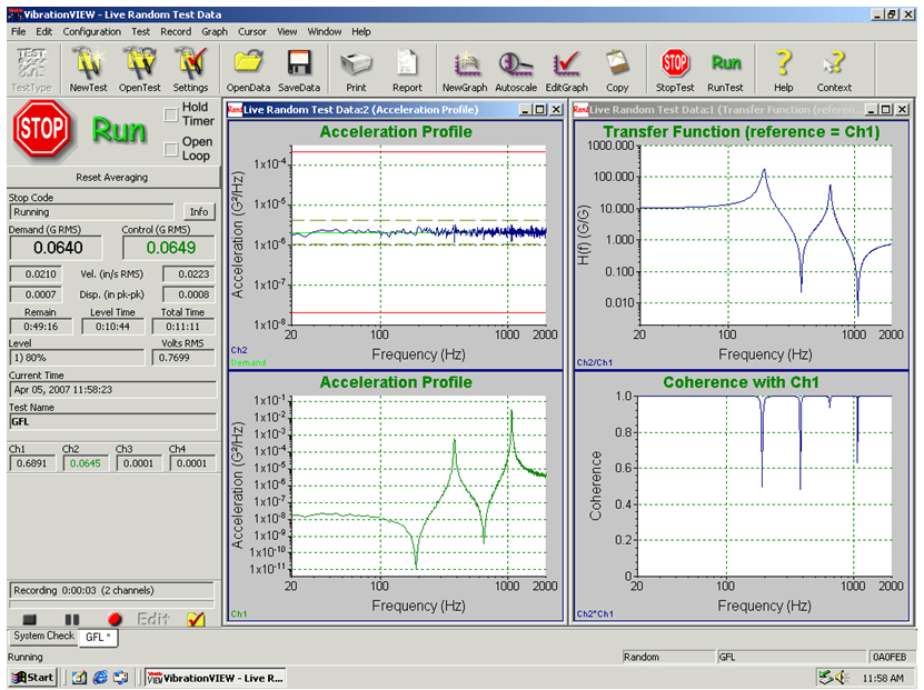
Figure 19. Closing the loop around a challenge filter with the VR 8500 using 800 lines of resolution.
Figure 19 illustrates a successful control lock on a challenge filter using a VR8500 with 800 lines of control, with all Control lines within ±3 dB of the Demand line. From this figure, one could be led to believe that the controller has passed this test. However, the challenge filter has a notch at 380 Hz with a bandwidth of only 0.35 Hz. The control bandwidth of 2,000Hz divided by 800 lines of control gives a controller line resolution of 2.5Hz. Knowing this, we recognize it is impossible for any controller to properly control this filter with only 800 lines! Adding an external analyzer to monitor the Drive and Control signals is probably prudent for independent validation of any loop-back test. However, in this particular case, we see that depending entirely upon an instrument to analyze its own worth is a serious error. In lieu of a stand-alone analyzer, you might substitute the use of a digital recorder (or recording software using the controller’s hardware) and offline analysis using software such as MATLAB®.
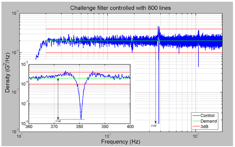
Figure 20. 800-line Control signal spectrum analyzed by an external analyzer with more resolution.
Figure 20 shows the Control signal as analyzed independently using a high-resolution FFT, with a line resolution of 0.08Hz. When analyzed independently we can see that the Control signal actually has more than 20 dB of error around the notch, far beyond the 3 dB the controller display reveals! From this, we can see that any challenge filter test must be verified using an independent analyzer. Simply relying on the controller’s display allows the controller imperfections to hide the true errors present in the signal.
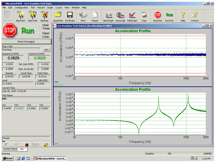
Figure 21. Closing the loop around the challenge filter with 13,000 lines of resolution.
To properly control this test we need a line resolution of 0.35Hz or better. This can be achieved by increasing the number of lines resolution employed by the controller. Figure 21 illustrates a successful control lock on a challenge filter using a VR 8500 with 13,000 lines of control, with all Control lines within ±3 dB of the Demand line. Figure 22 shows the independent analysis of this test, demonstrating proper control of this filter using 13,000 lines, with a maximum error of less than 2 dB.
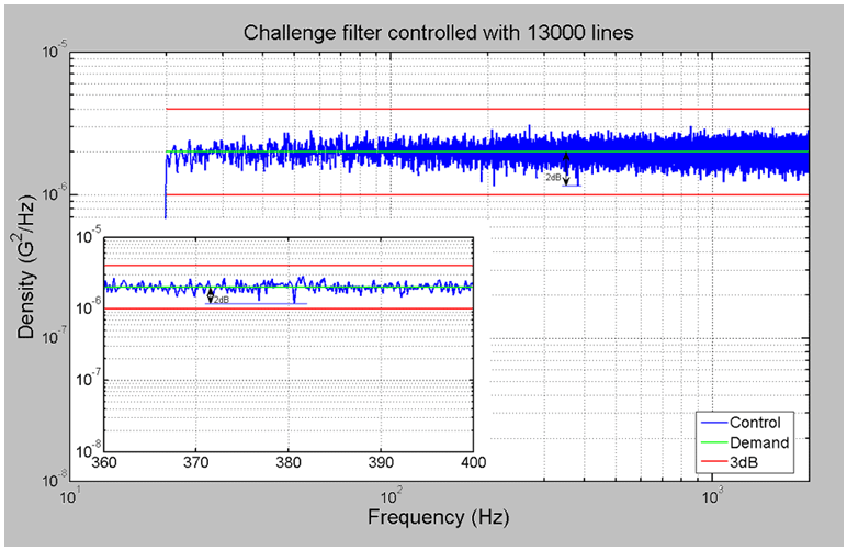
Figure 22. 13,000-line Control signal spectrum analyzed by an external analyzer.
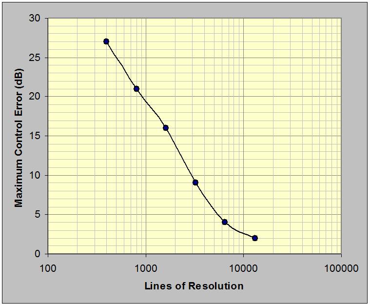
Figure 23. Maximum loop error versus random control resolution shows that at least 8,000 lines of resolution are required to hold the challenge filter in control within ±3 dB over the NAVMAT band.
Figure 23 presents a summary of worst-case loop error as a function of control resolution. In all cases, the worst error occurred at the 380 Hz filter notch. This investigation disclosed that at least 8,000 lines of controller resolution are required to control this challenge filter within ±3 dB over the 20 to 2,000 Hz NAVMAT bandwidth.
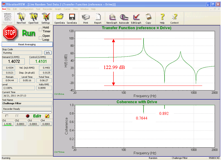
Figure 24. 13,000 line transfer function of the challenge filter shows over 120 dB of dynamic range on the VR9500; the corresponding coherence function indicates a clean measurement.
Figure 24 presents the transfer and coherence functions of the filter from the test of Figure 21. The dynamic range of the test is read from the amplitude extremes of the transfer function. The high coherence values at each transfer function peak and valley indicate clean control and linear filter behavior. Proponents of this test claim the dynamic range of the controller can be determined by taking the ratio of the maximum drive output to the minimum drive output. In the above test, we see the VR9500 demonstrates greater than 120 dB in this test, which corresponds to the dynamic range of the challenge filter. However, this test isn’t truly testing the dynamic range.
In fact, a 16-bit controller with 13,000 lines can also successfully demonstrate greater than 100 dB of dynamic range using this test, even though the true dynamic range of a perfect 16-bit converter is only 96 dB. To understand how this can be, consider that when running the challenge filter test the drive output from the controller must be the inverse of the filter transfer function to get a flat spectrum output from the filter. The notch in the filter transfer function will correspond to a very narrow peak in the required drive output. The maximum value of that peak is measured in V2/Hz, where the Hz portion is determined by the bandwidth of the peak. It follows that the maximum V2/Hz value can be increased without increasing the signal level simply by reducing the bandwidth.
In the sample case examined here, the highest peak has a 2.5 Hz bandwidth. If we assume a 1 VRMS signal with half of the total signal concentrated in this peak, then we would expect the V2/Hz level to be (0.5 V)2/(2.5 Hz) = 0.1 V2/Hz. Indeed, when scaled to a 1 VRMS level, we find the drive spectrum has a peak of 1 x 10⁻¹ V2/Hz. On the lower end, a 16-bit converter with ±10V range has a quantization noise floor of 8.8 x 10⁻⁵ VRMS, or 3.1 x 10⁻¹² V2/Hz. Taking the ratio of these two numbers, we see a 105 dB range can be shown with this test on a 16-bit system that we already know cannot exceed 96 dB of true dynamic range! For this reason, the challenge filter test, while useful to exercise the control loop and line resolution, should not be used as a measure of dynamic range.
Sine Algorithm and Output Test Using a High-Q Filter to Simulate a Shaker and Structure
The challenge filter may also be used in the setup in Figure 18 to measure dynamic range with a swept-sine test. For this test, a flat Demand amplitude is set, and the sine frequency is swept through the peaks and notches of the challenge filter. The implication of this is only the dynamic range of the control loop and the controller output signal are tested. Since the controller input is specified to maintain one amplitude level for the duration of the test, the dynamic range of the controller input remains untested. This test measures the relative values of the largest achievable output, which is required at the lowest notch in the filter transfer function, to the smallest achievable output (i.e. just above the noise floor) at the frequency of the highest peak in the filter transfer function.
Again, recall that to measure the dynamic range the test signals must be carefully crafted such that the highest output corresponds to the maximum range of the system. To successfully run this test, the loss at the lowest notch must be known in advance. For the sample case here, the filter transfer function has a 50dB loss at the lowest notch, so the demand level must be at least 50dB lower than the maximum achievable output voltage. For a controller with a 10 V maximum voltage, we choose a demand level of 0.01 VPEAK, or 60dB below the maximum.
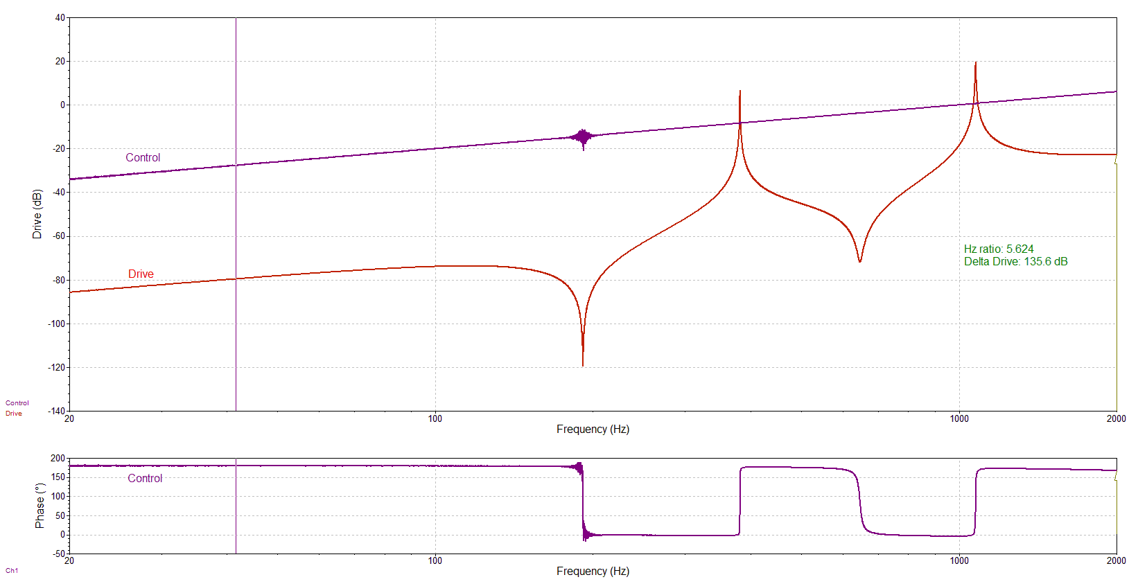
Figure 25. VR9500 Control and Drive signals during a swept-sine test; dynamic range exceeds 135 dB. The test profile has a change in demand amplitude (0.02 V to 2 V) because the dynamic range of VR9500 exceeded the dynamic range of challenge filter.
Figure 25 illustrates a swept-sine test using a constant amplitude of 0.01 VPEAKdemand. Note clearly evident Drive signal swings of 135 dB.
Conclusions
Eight tests of various aspects of the controller dynamic range have been demonstrated and discussed. The two-tone input and single-tone output tests, while useful for measuring harmonic distortion, were demonstrated to be poor measures of dynamic range. Their results depend more on the length of the FFT used for analysis than on the actual dynamic range of the device. The effective bits test was also presented. This test, while difficult to perform, does give a good measure of the signal-to-noise ratio of the system.
The use of a closed-loop random control challenge filter which simulates a lightly-damped system was also discussed. This test was shown to be prone to incorrect evaluation unless the results are verified independently from the controller’s display. It also provides an inaccurate, and inflated, measure of the dynamic range of the system. This test is useful for exercising the control loop in a realistic manner and is a good test of the line resolution of the controller. However, the dynamic range numbers given by this test can be more than 10 dB greater than the true dynamic range of the system, so this test should not be used as a measure of dynamic range.
Three loop-back tests were discussed, which test the controller inputs and outputs simultaneously, without requiring any external equipment. These three tests are simple to perform and combined give a good insight into the true capabilities of the controller.
At heart, the limits of a controller are determined by the maximum signal level, the noise floor, and the harmonic distortion characteristics of the system. The various measures of dynamic range will depend on these characteristics, but as was shown in this paper, dynamic range measurements can vary widely depending on how it is measured, and who is doing the measurement. Because of this, comparisons of controllers using dynamic range numbers are difficult at best. For unbiased comparisons, it is better to compare the maximum signal level, the noise floor, and the harmonic distortion characteristics of the systems.
Appeared in: Sound & Vibration Magazine, August 2007 pp 12-20.