ObserVIEW’s custom math and statistics capabilities are one of the many reasons why engineers download this analysis software program. By adding a math or statistics trace to a graph, engineers can calculate individual values for their analysis for the purpose of:
- Finding values to meet test standard requirements
- Interpreting data specific to the application
- Reporting more detailed results
The following text discusses several applications of ObserVIEW’s statistics graph traces, although there are countless potential uses. To learn more about math traces, visit 40 Uses for Math Traces in ObserVIEW.
Statistics Graph Traces
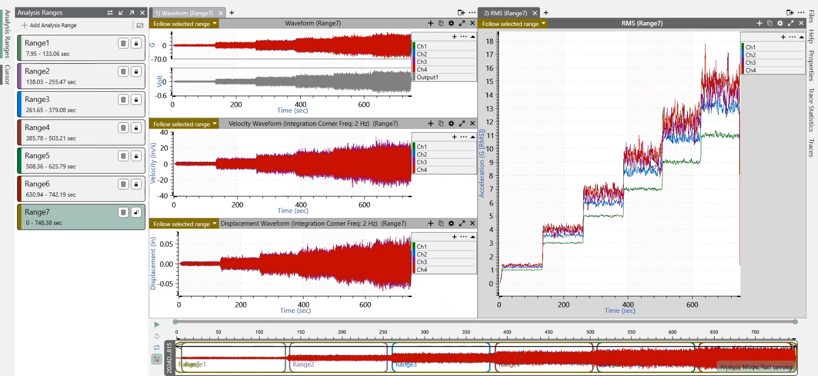
In ObserVIEW versions 2024 and newer, users can generate graphs for statistical analysis. Compared to cursors, which display data values at a specific location/range, graph traces allow the user to review statistics over time and compare the statistical behavior of multiple data sets.
Engineers can plot the following statistics over time for acceleration, velocity, or displacement data:
- Root-mean-square (RMS)
- Mean
- Variance
- Standard Deviation
- Skewness
- Kurtosis
- Maximax
- Minimum
- Range
- Crest Factor
Applications of Statistics Graph Traces
Extreme Values
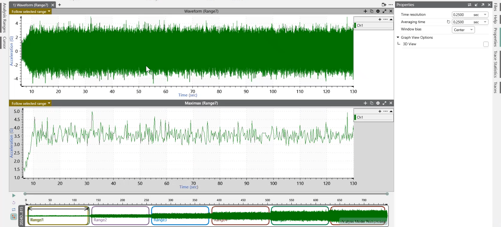
Users can evaluate the minimum, maximum, maximax, and range statistics to understand the extremes of a waveform.
Applications of Calculating Extreme Values in Data
- Verify that the maximum/minimum vibration levels meet design tolerances/test standards/safety compliance standards
- Identify minimum vibration levels during stable operation for benchmarking
- Determine natural frequencies by identifying the maximum responses in frequency-domain data
- Determine anti-resonances (minimum responses) for damping strategies
- Identify peak stress points to ensure materials can withstand extreme conditions
- Search for outliers in a batch test of components
Mean
The mean, or average, can indicate an offset in the data, meaning a shift from the expected zero point or baseline value. As the mean measures the central tendency of the data, it can help identify a data offset, drift over time, or DC content.
An offset in data can indicate:
- Baseline drift during longer tests, such as temperature-induced drift in accelerometers
- Misalignment of sensors or calibration errors
- DC bias in electrical signals from piezoelectric sensors
- Environmental noise interference
Variance
Variance describes the spread of data around its center (mean). A smaller variance indicates that the data is likely more stable with fewer extreme peaks. A larger variance can indicate rattle, shock, or another extreme event compared to the center of the data.
Applications of Calculating Variance in Data
- Evaluate product durability – excessive variance can indicate potential failure points
- Detect structural fatigue – monitoring variance in stress or strain measurements over time can help predict areas of fatigue
- Tune isolation systems – measuring variance can help optimize damping systems and minimize excessive movement
- Perform quality control – comparing variance between production samples helps ensure consistent performance across a batch of components
Standard deviation and RMS often serve the same purpose as variance. If the mean of the data is centered on zero, these values will be nearly identical. If not, the standard deviation will show the dispersion of data centered on the mean, and the RMS will relate to the overall energy.
Skewness
Skewness is a statistical moment that generally shows if data is more positive or negative. This information can be used to identify a potential offset or deviation from normal distribution.
Most vibration data sets are centered around 0. If data are skewed, it can indicate issues with data or imbalances in the system.
When comparing environments, the skewness time-history waveform can show the waveform’s stability through the duration of the event. A relatively flat line in the skewness time-history graph indicates that the data are stable across the recording. Variations indicate shifts, noise, rattles, or other deviations throughout the recording.
Kurtosis
Kurtosis is a statistical moment that describes the “peakiness” of a random waveform. Normally distributed Gaussian vibration has a kurtosis value of 3.
However, real-world data are often non-Gaussian. The contribution of these higher peaks to overall damage is important to understand when analyzing data and comparing environments.
Applications of Calculating Kurtosis in Data
- Identify high-amplitude peaks that may contribute disproportionately to fatigue damage
- Compare kurtosis values across different operating conditions to assess the effect of extreme peak events
- Confirm that a test profile accurately replicates the non-Gaussian characteristics of real-world environments by comparing kurtosis values
Crest Factor
The crest factor is the ratio between a peak value and RMS. This value is often used to understand the “peakiness” of a data set compared to normal distribution. It can highlight shock events or indicate an issue.
The crest factor measures how much “impact” occurs during a recording and can identify these events better than an FFT in cases of non-periodic impacts. Engineers can use a crest factor time history to measure the wear on a component (such as a bearing or gear).
Statistics Trace Properties
Statistics traces are calculated as rolling windows.
The “Averaging time” property determines the duration of the rolling window used to calculate the statistical value, similar to the degrees-of-freedom property in PSD calculations.
A longer averaging time results in a wider window, typically creating a smoothing effect. Combining a wide window and a short time resolution will result in a smoother data set.
The “Time resolution” property determines the time step between windows, which equates to the distance between the measurements on the graph. If the time resolution is shorter than the averaging time, there will be some amount of overlap in the data analyzed for each sample. The effect is similar to the percentage overlap property in PSD calculations.
Download ObserVIEW
Download a free demonstration of the ObserVIEW analysis software and begin editing and analyzing waveforms straight away. Interested in learning more? Visit the software page.