The math traces feature in the ObserVIEW software adds a user-defined math expression to a time or frequency graph. Math traces allow the user to plot custom math operations not defined by the software’s current graph types.
Math traces applied to a time waveform graph are math channels. Math channels are unique in that the user can create spectrum traces from them, such as an FFT or PSD.
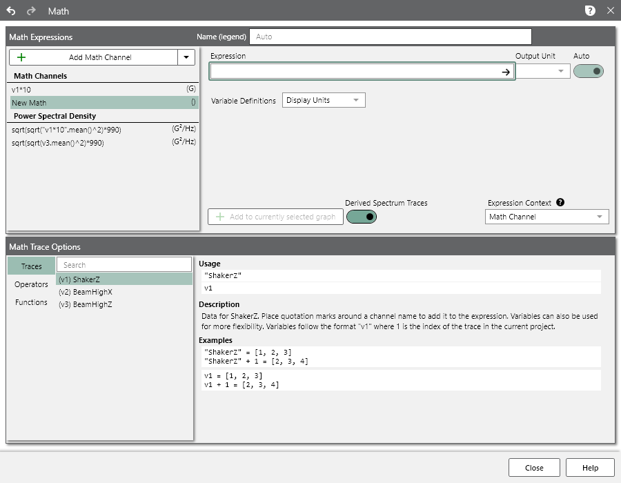
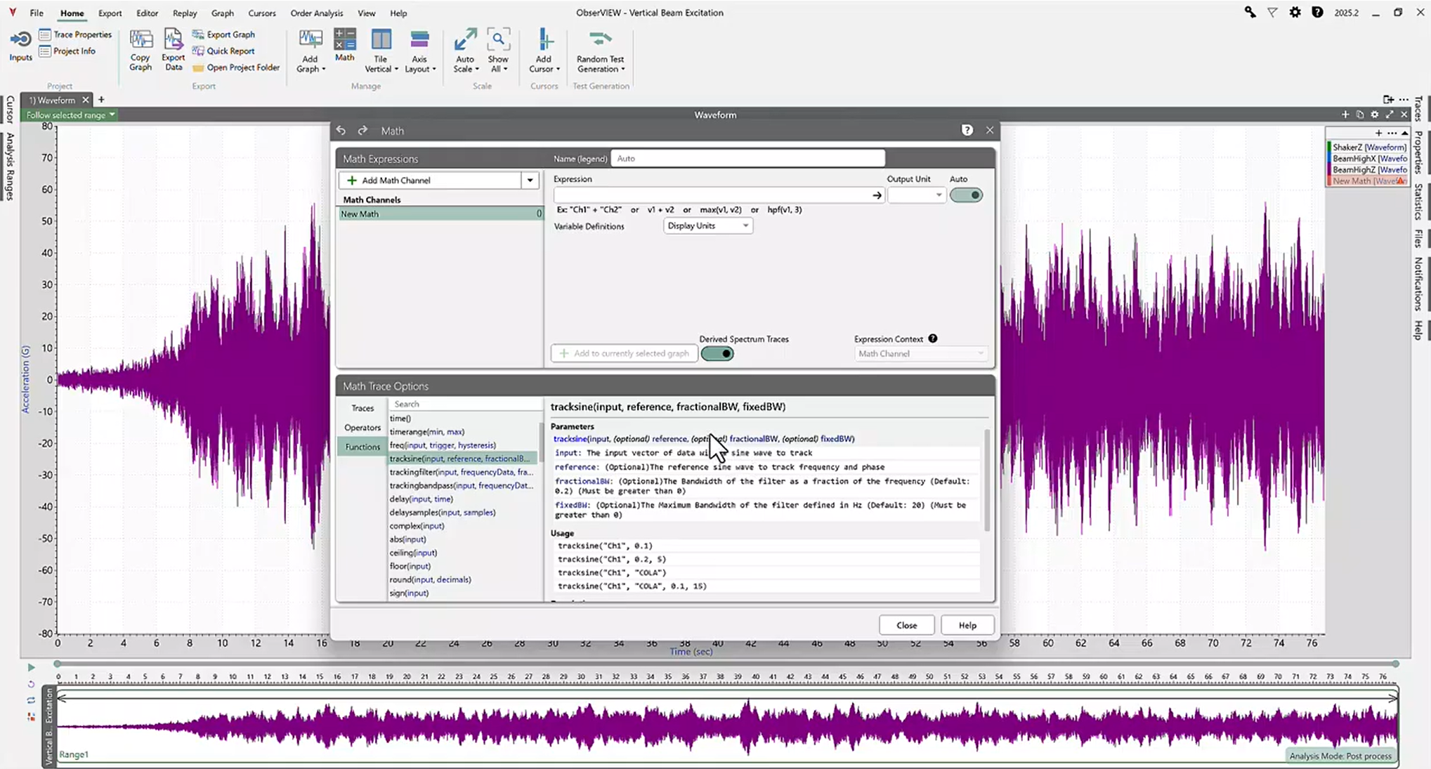
The Math function is a free entry field that builds a trace by applying functions/operators to existing trace data. To add a math trace to a graph, select the Math button on the ribbon or right-click any non-spectrogram graph and select Add Math Channel/Trace.
Reference
The user can reference a trace or channel using a variable definition (v1, v2, etc.) or quotations around the name (ex. “Ch1”).
Functions
ObserVIEW can apply two types of functions to existing trace data.
The first uses a trace or set of traces as a parameter to produce a trace as an output. For instance, Max(v1, v2) produces a new trace where the value at each frequency point is the maximum value of the input traces at that frequency.
The software applies the second function type to a trace as a dot operation and produces a single value. For instance, v1.Max() produces a single value: the maximum of all values in v1. If the result of an expression is a single value, the software will produce a trace repeating that value (a straight line).
Limitations
Math traces do not work on spectrograms or random test generation graphs.
40 Uses for Math Traces
Math Traces
- Envelope multiple PSD traces
To find the maximum possible PSD from three different sensors:
- Add a math trace to a PSD graph.
- Enter the expression: max(v1, v2, v3)
- Ensure that the variable definition units match each other and the output unit.
Each point on the resulting math trace is the maximum value of the input PSD traces at the given frequency.
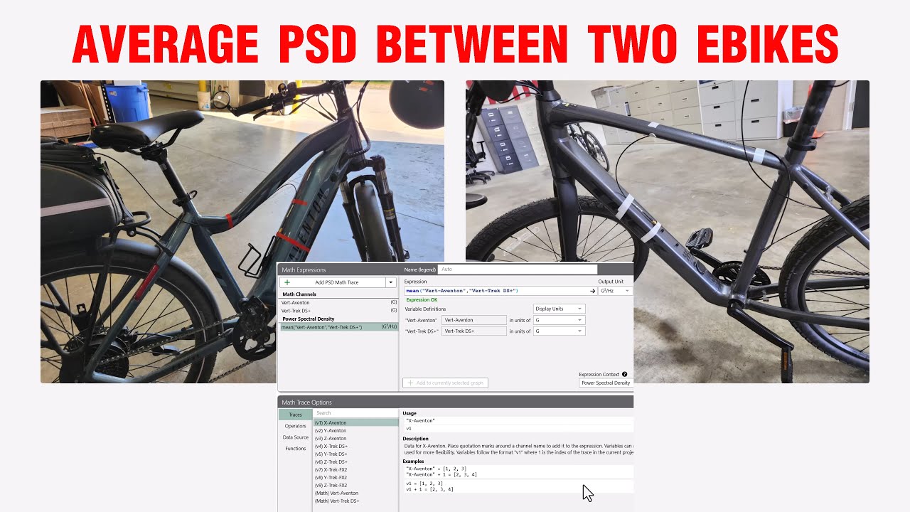
- Create an average PSD trace
An average PSD may be necessary for average test control. To find the average PSD from three different sensors:
- Add a math trace to a PSD graph.
- Enter the expression: mean(v1, v2, v3)
- Ensure that the variable definition units match each other and the output unit.
Each point on the resulting math trace is the average value of the input PSD traces at the given frequency.
- Scale a trace by a constant factor
To multiply every value of a trace by 2.5:
- Add a math trace to a graph.
- Enter the expression: 2.5 * v1
- Set v1 to the trace of interest.
- Ensure that the variable definition unit matches the output unit.
This scaling can be applied to time waveforms and frequency traces. Applying it to a time waveform will automatically create the derived frequency traces for the resulting waveform.
- Find the ratio of two FFTs
- Add a math trace to an FFT graph.
- Enter the expression: v1 / v2
- Set v1 and v2 to the proper traces.
- Ensure that the variable definition units match each other and the output unit.
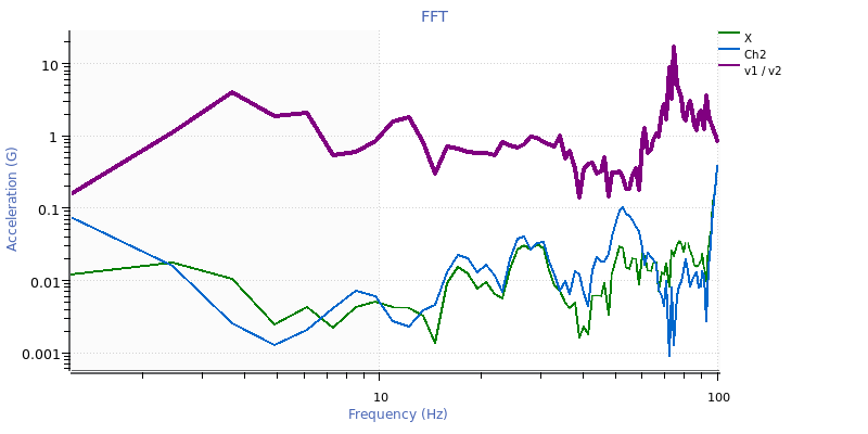
FFT ratio math trace.
- Find the absolute acceleration or total power of a triaxial accelerometer
- Add a math trace to a frequency graph.
- Enter the expression for the trace type:
- For FFT/octave/etc.: sqrt(sum(v1^2, v2^2, v3^2))
- For PSD and CSD: sum(v1, v2, v3)
Note: Amplitude traces use a vector sum because they are directional. Power traces such as PSD are not directional, so they use a standard sum.
Note: For CSD traces, a complex projection must be specified, such as mag(v1).
- Set v1, v2, and v3 to the acceleration channels of the triaxial sensor.
- Ensure that the variable definition units match each other and the output unit.
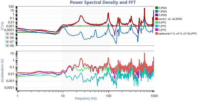
Absolute acceleration for a triaxial sensor on a PSD and FFT graph.
- Transmissibility of an average control channel
Some applications require an average control channel, where the control is assumed to be the average of multiple channels. In this case, a transmissibility trace cannot be properly calculated using a transmissibility graph. However, a math trace can be used to calculate the transmissibility. In this example, there are four channels that make up the average control, and the acceleration channels were recorded in units G:
- Add a math trace to a PSD graph.
- Enter the expression: sqrt(v5 / mean(v1, v2, v3, v4))
- Set v1, v2, v3, and v4 to the control channel traces, and set v5 to the desired trace to calculate transmissibility.
- Ensure the variable units are correct, and set the output unit to G/G.
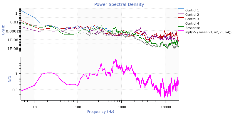
Transmissibility of an average control channel.
- Find the relative power between two waveforms for a given time period
- Add a PSD graph.
- Add a math trace to the PSD.
- Enter the expression: v1.rms() / v2.rms()
- Set your variable definitions for v1 and v2 to the channels being compared.
The software will graph a line at the ratio between the power levels of the two channels for the selected PSD data range. Set the data range to the time period of interest.
- Determine the maximum shock response for different environments
- Record data in various environments for the same shock event.
- Overlay the event recordings to produce a single ObserVIEW project.
- Add a shock response spectrum (SRS) graph.
- Add a math trace to the SRS.
- Enter the expression: max(v1, v2, v3)
- Ensure that the variable definitions are correct and that the input units match the output unit.
The resulting trace on the SRS graph is the envelope of the SRS traces from the different environments.
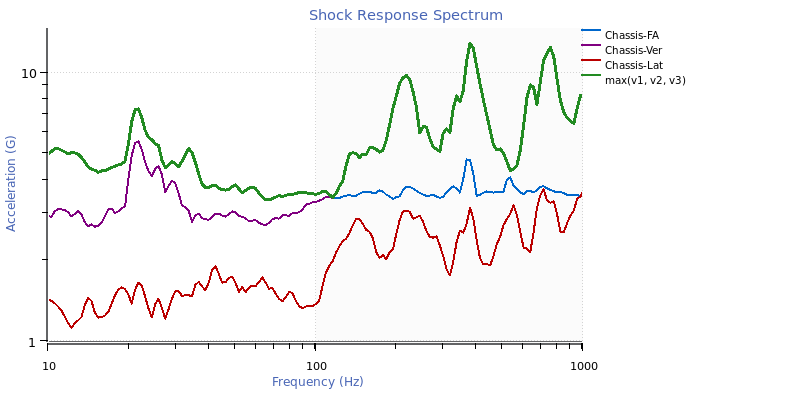
Maximum SRS math trace.
- Average the transfer function for multiple channels
If multiple channels have a similar event recorded at the same time, or if events have been overlaid into a project, a math trace can average the transfer functions. For example, the following expression will find the average magnitude of four transfer functions: mean(mag(xfer(v1)), mag(xfer(v2)), mag(xfer(v3)), mag(xfer(v4)))
- Calculate a narrowband RMS
A math trace can calculate the root-mean-square (RMS) for a frequency range. On a frequency graph, such as a PSD, identify the low and high frequencies of interest. Then, set the frequency range, and add a math trace to find the RMS. For example, the following expression will find the RMS for a frequency range of 50 to 400Hz: (v1 * freqrange(50, 400)).rms()
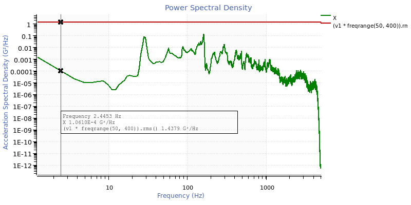
Narrowband RMS math trace.
- Convert a trace to decibels
To calculate the decibel value for a trace:
- Add a math trace to a graph.
- Identify the reference value scale factor. This value defines 0dB. For this example, the reference value is 20μPa.
- Use a conversion equation appropriate for your trace type.
- For FFT/octave/etc.: 20 * log10(v1 / 20)
- For PSD and CSD: 10 * log10(v1 / 20)
Note: Values are multiplied by 20 for amplitude traces, and values are multiplied by 10 for power traces.
Note: For CSD traces, a complex projection must be specified, such as mag(v1).
- Select a trace conversion.
- Ensure that your input unit matches the dB reference unit. The output unit should be set to a custom unit for decibels but may also be graphed on the same axis as the original trace by setting the output unit to the current display unit.
- Amplify a trace by a specific decibel value
To add a decibel (dB) value to a trace’s values, the trace must be converted to dB, modified, and then converted back. The following example adds 50dB to the trace. The math is simplified in the example expressions below:
- For FFT/octave/etc.: v1 * 10^(50 / 20)
- For PSD and CSD: v1 * 10^(50 / 10)
Note: For CSD traces, a complex projection must be specified, such as mag(v1).
- Add a coherence mask to a transfer function
A transfer function is only useful at frequencies where the coherence is sufficiently high. Math traces can highlight these frequency ranges. To add a coherence mask to a transfer function graph:
- Add a math trace to a transfer function graph. Disable the visibility of all the traces on the graph except one for the coherence mask.
- Enter the expression: mag(coh(v2))
- Ensure that the variable definitions are correct. v2 is the trace for the coherence mask.
- Add another math trace, and enter the desired coherence threshold as the expression. In this example, 0.8 is the limit.
- Change the output unit of the math trace to Coherence. Close the math trace dialog.
- Right-click on the 0.8 trace in the legend and select “Set as Tolerance Min.”
- Right-click on the mag(coh(v2)) math trace in the legend and select “Set as Tolerance Reference.”
- Disable the visibility of the two math traces on the graph.
The resulting graph is a transfer function where the background is highlighted green at frequencies where the coherence is higher than the defined threshold.
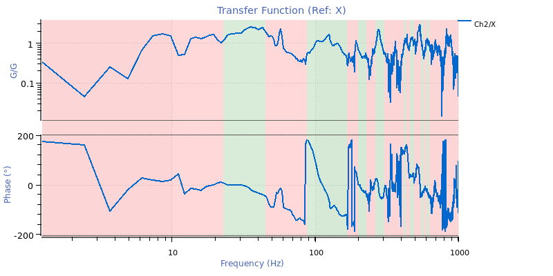
Coherence mask math trace.
A coherence mask can also be accomplished with a slightly different math trace: mag(v2) * ((mag(coh(v2)) > 0.8)
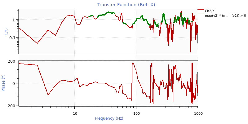
Coherence mask math trace.
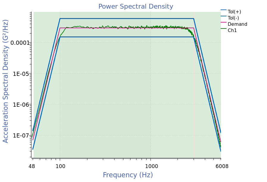
- Add tolerance lines centered about a pasted demand trace
When analyzing random waveform data, it is helpful to evaluate if data are within tolerance. In this example, math traces will function as ±3dB tolerance lines.
- Create a demand line in a spreadsheet or text editor. The following example defines a target demand line at 1gRMS from 100 to 3,000Hz.
| Hz | G2/Hz |
| 50 | 7.00E-08 |
| 100 | 3.00E-04 |
| 3000 | 3.00E-04 |
| 6000 | 6.00E-08 |
- Copy and paste the demand line onto a PSD graph and rename the trace to “Demand.”
- Add a math trace to the graph and name it “Tol(+)”: “Demand” * 10^(3 / 10)
Note: “+3” in this expression creates a +3dB copy of the Demand trace.
- Duplicate this math trace (right-click > duplicate), change the positive value (+) to a negative one (-), and name it “Tol(-)”: “Demand” * 10^(-3 / 10)
Note: “-3” in this expression creates a -3dB copy of the Demand trace.
- Optional: add tolerance highlighting.
- Right-click Ch1 > “Set as Tolerance Reference”
- Right-click Tol(-) > “Set as Tolerance Minimum”
- Right-click Tol(+) > “Set as Tolerance Maximum”
- Convert an octave-filtered trace to a PSD trace
A specification might call for a PSD computed with filtered octave data. To create this trace:
- Add a PSD graph.
- Add a math trace to the PSD.
- Change the expression context of the math trace to “Octave.”
- Enter the following expression, which assumes 1/6 octave spacing. Replace the 6 with the octave spacing property chosen in the octave trace options: v1^2 / ((10^(0.5 * 0.3 / 6) – 10^(-0.5 * 0.3 / 6)) * freq())
Note: “0.3” represents how octave spacing is defined as the nominal frequency times multiples of 10^0.3, and “±0.5” represents going forward and backward half a bin to get the bin width.
- Ensure that v1 is set to the proper trace, and set the output unit to the acceleration spectral density unit g2/Hz.
- Set the Weighting option in Octave Properties to “None (Z).”
Note: for Live Analyzer, set the Octave Integration Time property in Trace Properties to a longer time, such as 10 seconds, to better relate to PSD averaging with large degrees of freedom (DOF) (ex: 60 DOF is about 10sec averaging at 1Hz resolution).
Below is a traditional FFT-based PSD trace compared to an octave trace converted to PSD units.
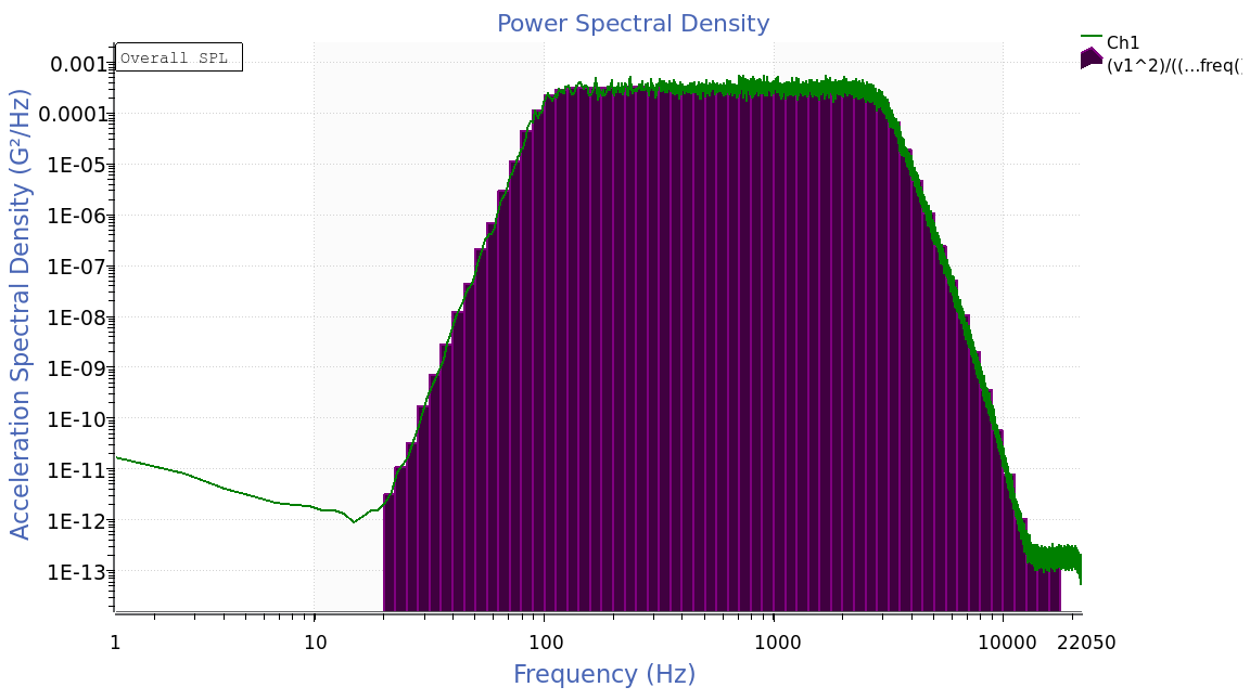
PSD trace from an octave trace.
- Integrate or differentiate a frequency trace (convert AVD)
AVD integration and differentiation can be performed on frequency traces using division and multiplication as opposed to AVD filters in the time domain. To perform integration or differentiation on frequency traces:
- Add a math trace to a frequency graph.
- Use the appropriate conversion expression for the desired AVD conversion. In this example, the order of integration/differentiation is 2, representing double integration/differentiation. For example, a 2nd order integration on acceleration data will produce displacement data. The last 2 in each expression is the order value:
- For integration on FFT/octave/etc.: v1 / (2 * pi * freq())^2
- For differentiation on FFT/octave/etc.: v1 * (2 * pi * freq())^2
- For integration on PSD or CSD: v1 / ((2 * pi * freq())^2)^2
- For differentiation on PSD or CSD: v1 * ((2 * pi * freq())^2)^2
Note: The integration/differentiation dividend/product is squared for power traces.
Note: For CSD traces, a complex projection must be specified, such as mag(v1).
- Set v1 to the desired trace to integrate/differentiate.
- Ensure that the variable definition units and output unit are set to SI (m, m/s, m/s2, etc.). For PSD or CSD, set the output unit to the correct spectral density SI unit for the given conversion, creating a new unit if necessary. For instance, after converting an acceleration spectral density to displacement spectral density, the output unit is set to m2/Hz.
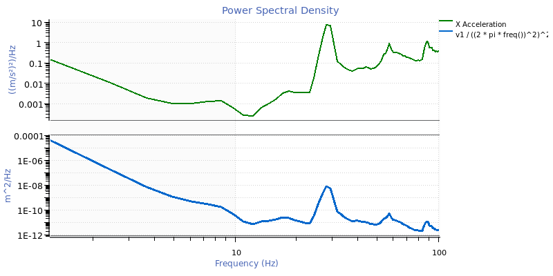
Integration of acceleration channel.
- Convert power traces (PSD or CSD) to amplitude
If a power trace has squared units in the numerator (such as G2/Hz), then math traces can be used to convert it from power units back to amplitude (such as G):
- Add a math trace to a PSD or CSD graph.
- Enter the expression: sqrt(v1 * v1.df())
Note: v1.df() is equal to the frequency resolution of the trace v1.
Note: For CSD traces, a complex projection must be specified, such as mag(v1).
- Ensure that v1 is set to the proper trace and has the proper unit. For CSD traces, ensure that the reference trace has the same unit.
- Set the output unit to the corresponding amplitude of the spectral density unit (for example, if the PSD unit is g2/Hz, then the math trace output unit should be g).
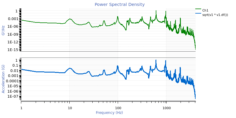
Power spectrum converted to amplitude math trace.
Math Channels
- Scale a trace by a constant factor
To multiply every value of a trace by 2.5:
- Add a math trace to a graph.
- Enter the expression: 2.5 * v1
- Set v1 to the trace of interest.
- Ensure that the variable definition unit matches the output unit.
This scaling can be applied to time waveforms and frequency traces. Applying it to a time waveform will automatically create the derived frequency traces for the resulting waveform.
- Find the difference between two waveforms
- Add a math trace to a waveform graph.
- Enter the expression: v1 – v2
- Set v1 to the minuend trace and v2 to the subtrahend trace.
- Ensure that the variable definition units match each other and the output unit.
- Add a constant reference
A constant value can be entered into the expression to create a constant reference trace. For example, the expression 5 with the output unit G will create a trace with a value of 5G at every time value.
- Apply IIR low-pass, high-pass, and band-pass filters to individual traces
When analyzing shock waveforms, it can be critical to filter high and/or low-frequency data. ObserVIEW can universally apply low- and high-pass IIR filters, but a math trace can filter a channel independently. For example, observe how a low-pass filter at 2kHz cleans up a shock waveform:
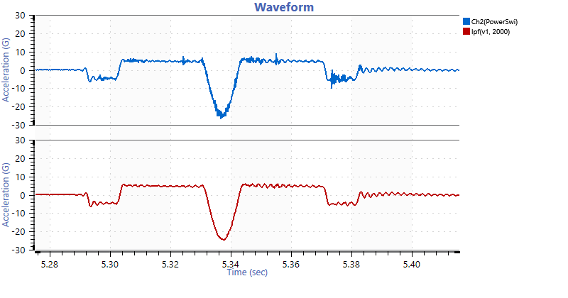
A low-pass filter at 2 kHz.
To add this filter type:
- Add a math channel to a waveform graph.
- Enter the expression: lpf(v1, 2000)
This expression adds a 6th-order Butterworth low-pass filter at 2,000Hz to the vector v1.
- Set v1 to the trace being filtered.
- Ensure that the variable definition unit matches the output unit.
Additionally, the hpf() function can create a high-pass filter. The lpf() and hpf() functions can be applied together to create a band-pass filter: lpf(hpf(v1, 10), 2000)
This expression adds a high-pass filter at 10Hz and a low-pass filter at 2,000Hz to the vector v1.
- Find the absolute acceleration of a triaxial accelerometer
- Add a math channel to a waveform.
- Enter the expression: sqrt(v1^2 + v2^2 + v3^2)
- Set v1, v2, and v3 to the acceleration channels of the triaxial sensor.
- Ensure that the variable definition units match each other and the output unit.
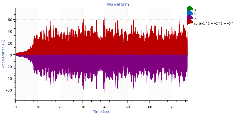
Absolute acceleration math trace.
- Rotate triaxial sensor channels to new directions
During recording setup, triaxial sensors sometimes need to be mounted off the desired axes due to space constraints. If the engineer knows the angle that the sensor is mounted on, they can adjust the axes’ direction of motion.
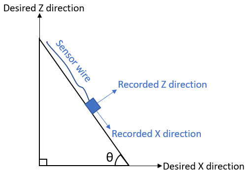
The angle from horizontal for the recorded X-axis.
If the recorded X direction is angled down (as illustrated in the image above), to perform a single rotation of the data about the Y axis (i.e., the Y data stays the same and the X and Z data are adjusted):
- Determine the angle from horizontal for the recorded X-axis. This angle is θ (radians).
- Add a math channel to a waveform graph.
- Enter the expression for the new Corrected X channel: “X” * cos(θ) + “Z” * sin(θ)
- Add another math channel to the waveform graph.
- Enter the expression for the new Corrected Z channel: -“X” * sin(θ) + “Z” * cos(θ)
These expressions change if the positive X or positive Z directions are reversed compared to the image above. In this case, the θ in each expression will need to be multiplied by -1 to account for the direction change:
- New Corrected X channel: “X” * cos(-θ) + “Z” * sin(-θ)
- New Corrected Z channel: -“X” * sin(-θ) + “Z” * cos(-θ)
Note: If both the X and Z are reversed, use a positive θ value.
These operations can be combined to rotate the sensor data for a more complex setup that needs to rotate all three axes. As above, the angles may need to be multiplied by -1 depending on sensor orientation. The expression for a Z channel from a rotation by θ about the X axis followed by a rotation by φ about the Y axis is: “X” * sin(φ) – “Y” * sin(θ) * cos(φ) + “Z” * cos(θ) * cos(φ)

- Find the relative power over time between two waveforms
- Add a math channel to a waveform graph.
- Enter the expression: rms(v1) / rms(v2)
- Set your variable definitions for v1 and v2 to the channels being compared.
- Ensure that the variable definition units match each other.
- Calculate a jerk waveform from acceleration
To differentiate acceleration and produce a jerk waveform:
- Add a math channel to a waveform graph.
- Enter the expression: differentiate(v1, 1, 3000)
This expression will use an IIR filter to differentiate the trace selected for v1 one time, with a corner frequency of 3,000Hz. The corner frequency should be above the maximum frequency of interest.
- Set the working unit for the acceleration variable to m/s2 (SI units) and the output unit to m/s³. ObserVIEW doesn’t include jerk units by default, so adding a custom one in units settings may be necessary.
- Calculate angular acceleration from angular velocity
Similar to converting acceleration to jerk, a differentiation filter is used to differentiate angular velocity and produce an angular acceleration waveform:
- Add a math channel to a waveform graph.
- Enter the expression: differentiate(v1, 1, 3000)
This expression will use an IIR filter to differentiate the trace selected for v1 one time, with a corner frequency of 3,000Hz. The corner frequency should be above the maximum frequency of interest.
- Set the working unit for the velocity variable to rad/s (SI units) and the output unit to rad/s2.
- Calculate displacement from acceleration
To double-integrate acceleration and produce a displacement waveform:
- Add a math channel to a graph.
- Enter the expression: integrate(v1, 2, 3)
This expression will use an IIR filter to integrate the trace selected for v1 twice, with a corner frequency of 3Hz. The corner frequency should be close to 0.
- Set the working unit for the acceleration variable to m/s2 (SI units) and the output unit to m.
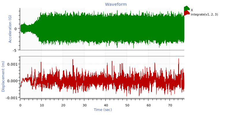
Double-integration math trace.
- Calculate angular acceleration and angle from two accelerometers
Consider a beam that rotates around a point “p” and is measured by two accelerometers that are “d” meters apart:
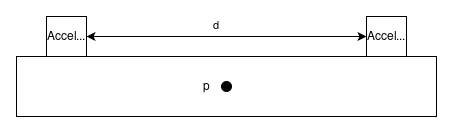
The accelerometers will measure the linear acceleration at their respective locations on the beam but not the angular acceleration.
The following formula calculates angular acceleration:
(1) 
Where α is the resultant angular acceleration in rad/s2, A1 is the linear acceleration of the first accelerometer (m/s2), A2 is the linear acceleration of the second accelerometer, and D12 is the distance between the two accelerometers in meters. A negative sign is placed in front of A2 as a correction because the A2 accelerometer is oriented in the same direction as A1.
In the example above, we can use a math trace. If the distance “d” were 3 meters, the following steps would calculate the angular acceleration:
- Add a math channel to a waveform graph.
- Enter the expression: (“Ch1” – “Ch2”) / 3
- Ensure that “Ch1” and “Ch2” have working units of m/s2 in the “Variable Definitions” section and that the output unit is rad/s2.
An integration filter can calculate the angle between the accelerometers, and a high-pass filter can smooth out the results. For example: integrate(hpf((“Ch1” – “Ch2”) / 3, 5), 2, 5)
- Combine signals from multiple force sensors
Math traces can combine the signals from any number of force sensors. Consider the following diagram:
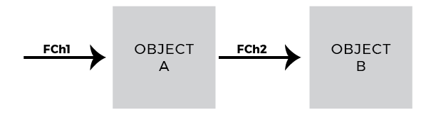
To find the magnitude of the forces applied to Object B:
- Add a math channel to a waveform graph.
- Enter the expression: sqrt(“Ch1″^2 + “Ch2″^2)
- Ensure that the input units match the output unit.
- Verify data are centered around zero in a controlled environment
The statmean() function computes the statistical mean of a waveform using an exponentially rolling window. It can be used to verify that a channel is centered at approximately zero: statmean(“Ch2(PowerSwi)”)
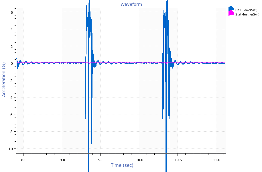
Statistical mean math trace.
- Calculate the standard deviation of data
A waveform with many shock events will have a high standard deviation, whereas a more consistent waveform will have a lower standard deviation: stddev(v1)
- Analyze a recording using kurtosis
Kurtosis over time can inform an engineer about the validity of a recording waveform.
- Add a math channel to a waveform graph.
- Enter the expression: kurtosis(v1)
- Make note of the output unit. If it is different from the display unit, the kurtosis level will be scaled to the display unit. To avoid confusion, set the output unit to the display unit for the given unit category.
- Observe the resulting kurtosis waveform for changes and unexpected levels. A few considerations:
- If the recorded data is Gaussian random, it should have a kurtosis level of around 3.
- If the recorded data has a kurtosis level of less than 3, then it likely has prominent patterns, such as sine tones.
- If the recorded data has many high amplitude peaks over the average, it will have a kurtosis greater than three. When reproducing this environment on a shaker using VibrationVIEW, it is suggested to use Kurtosion control.
- If the recorded data has extremely high kurtosis (>30), it is likely that there are data errors and/or discontinuities in the recording.
- Average sensors on the same axis
If using multiple sensors in the same axis direction, a math trace can calculate their average.
- Add a math channel to a waveform graph.
- Enter the expression: mean(v1, v2)
- Calculate the exponentially rolling RMS of a waveform
A math channel can find the rolling average power of the waveform, exponentially weighted towards more recent data. The decay time defaults to 2 seconds. A PSD or FFT cursor will also produce an RMS, but the value is distributed evenly across the data range for the FFT or PSD. In contrast, the rms() math trace function for waveforms will consider all previous values, but place a greater weight on more recent data. The rms() function is beneficial in comparing waveforms, as differences in phase between them will not have a significant impact on the comparison: rms(v1)
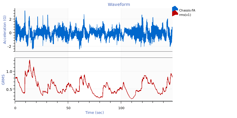
RMS math trace.
- Convert a trace to decibels
To calculate the decibel value for a trace:
- Add a math trace to a graph.
- Identify the reference value scale factor. This value defines “0dB.” For this example, the reference value is 20μPa.
- Use a conversion equation appropriate for your trace type.
- For waveforms: 20 * log10(abs(v1 / 20))
Note: For waveforms, the expression above will convert negative values to positive decibel values.
- Select a trace for conversion.
- Ensure that the input unit matches the dB reference unit. The output unit should be set a to custom unit for decibels, but may also be graphed on the same axis as the original trace by setting the output unit to the current display unit.
- Amplify a trace by a specific decibel value
To add a dB value to a trace’s values, the trace must be converted to decibels (dB), modified, and then converted back. In this example, 50dB will be added to the trace. This math is simplified in the following example: v1 * 10^(50 / 20)
- Fix data recorded in an incorrect unit
For example, the sensor sensitivity is 10mV/G, but the data was recorded with a sensitivity of 10mV/(m/s2). This can be solved by adding math trace v1 and manually selecting m/s2 as the variable unit. Then set the output unit to G. This redefines the channel unit to G while keeping the same values.
- Calculate the minimum, average, and maximum RMS acceleration levels between three channels
- Minimum: min(rms(v1), rms(v2), rms(v3))
- Average: mean(rms(v1), rms(v2), rms(v3))
- Maximum: max(rms(v1), rms(v2), rms(v3))
- Count the number of samples out of tolerance
A math channel with the cumulative sum cumsum() function can be used to count the number of samples that exceed a tolerance. For example, the following expression can produce a waveform that counts how many samples exceed a 100gRMS tolerance: cumsum(rms(v1) > 100)
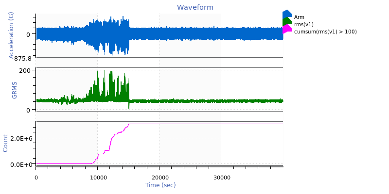
Cumulative sum math trace indicating how many samples of the acceleration waveform exceed a 100gRMS tolerance.
- Generate waveforms
Random waveform with an RMS of 1.0: randn()
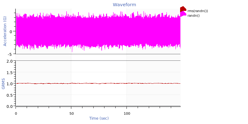
Random waveform with an RMS value of 1.
Sine tone with an amplitude of 5 and a frequency of 30Hz: 5 * sin(time() * 30 * 2 * pi)
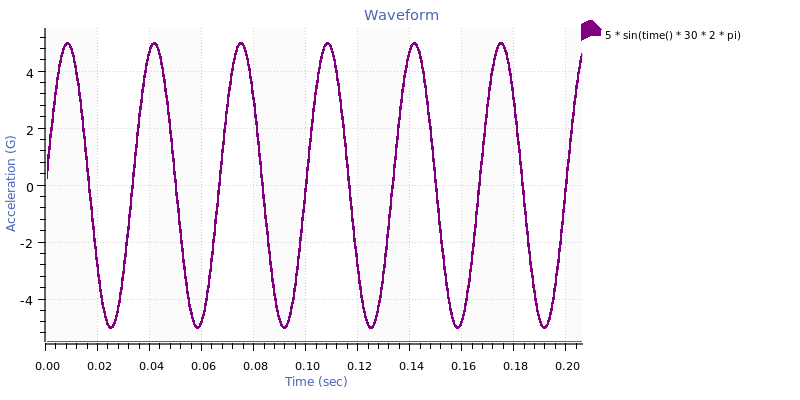
Sine tone.
Square wave with an amplitude of 5 and a frequency of 30Hz: 5 * (-1)^floor(2 * 30 * time())
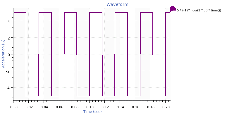
Square wave.
Sawtooth wave with an amplitude of 5 and a frequency of 30Hz: 5 * 2 * (30 * time() – floor(0.5 + 30 * time()))
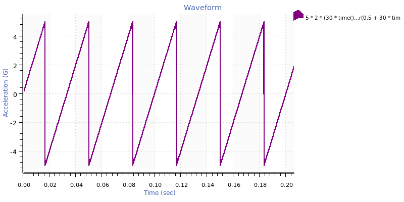
Sawtooth wave.
Triangle wave with an amplitude of 5 and a frequency of 30Hz: 5 * (2 * abs(2 * (30 * time() – floor(30 * time() + 0.5))) – 1)
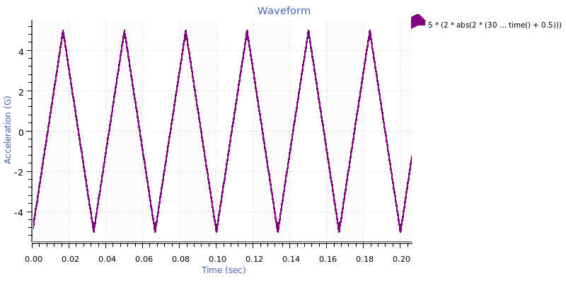
Triangle wave.
Sine sweep with log sweep rate from 3 to 100 Hz at 1 Hz/octave for 2.5 sec with an amplitude of 5: 5 * sin((2 * pi * 3 * 2.5) / ln(100 / 3) * (pow(e, time() / 5 * ln(100 / 3)) – 1))
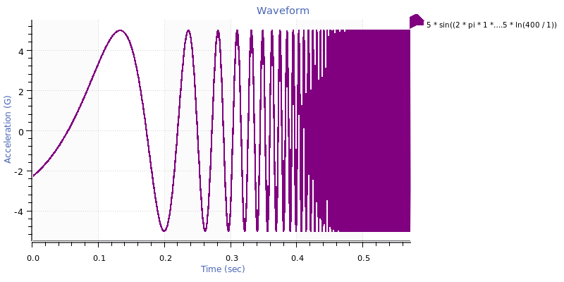
Log sine sweep.
Sine sweep with linear sweep rate from 3 to 100 Hz for 2.5 sec with an amplitude of 5: 5 * sin(2 * pi * (3 + (100 – 3) / (2 * 2.5) * time()) * time())
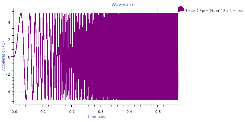
Linear sine sweep.
Sine tone at 30Hz with a phase shift of 1/3 pi radians in complex variable notation: imag(e^(i * 2 * pi * 30 * time()) * e^(i * 1 / 3 * pi))
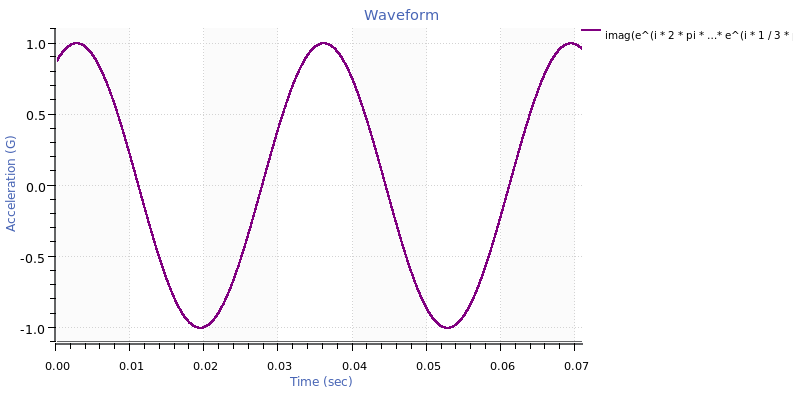
Sine tone with phase shift.
Cosine tone at 30Hz with an exponential decay factor of 5 in complex variable notation: real(e^(i * 2 * pi * 30 * time()) * e^(-5 * time()))
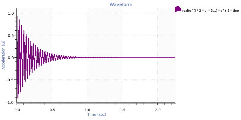
Cosine tone.
41. Analyze and Reprocess Sine Reduction Test Data
Math Channels includes expressions for post-process sine data analysis that simplify sine sweep data by breaking down the frequency and amplitude components of time-domain signals. This method provides clearer insights than traditional graphs like the FFT or transmissibility.
- freq(“Output”): Calculates the frequency of a sine tone signal in Output; “Output” can be replaced with the file’s sine tone reference channel
- tracksine(“Ch1”, “Output”): Tracks the Ch1 sine amplitude using the Output channel as a reference
- mag(tracksine(“Ch1”, “Output”)): Tracks the peak amplitude of the Ch1 tone over time
- phase(tracksine(“Ch1”, “Output”)): Tracks the phase shift between Ch1 and Output