Acoustic measurement allows engineers to assess the sound related to a device under test, predict operational environments, and address design problems. However, acoustic measurement does not contain frequency information, making it unsuitable for comparing sound and vibration. Vibration test engineers use a frequency analysis technique called octave analysis to identify an acoustic signal’s frequency content.
What is Octave Analysis?

Octave analysis groups a signal’s frequency range into octave “bands.” For commercial applications, engineers typically analyze the standard audible frequency range for humans (20-20,000Hz). For a given input signal, an octave plot indicates the loudness of each octave range, allowing engineers to target specific frequencies.
The software filters the signal and measures the sound pressure levels. As the human ear responds to frequency changes on a logarithmic scale, it typically spaces the octave bands logarithmically and measures the signal’s intensity in decibels (dB). The engineer can apply averaging and weighting to the frequency-domain content to correspond to their desired evaluation of sound.
The rest of this article will refer to the process of octave analysis in the ObserVIEW software, which uses standard methods.
Octave-band Filter
ObserVIEW’s octave-band filter separates a signal’s frequency range into bands with octave-spaced center frequencies. The filter accounts for the bandwidth, center frequency, and filter order. ObserVIEW generates octave bands with an 8th-order filter to meet IEC 61260-1 Class 1 filter specifications.
The octave band spacing property determines the bandwidth. With 1/1 octave spacing, each band is one octave, meaning each center frequency is twice the previous band’s center frequency.
Fractional octave analysis further separates each octave. For 1/3 octave spacing, each octave has three bins; for 1/6, each octave has six bins, etc. Fractional octave analysis allows the engineer to select a frequency resolution suited to their signal of interest.
Calculating Octaves
The definition of an octave varies depending on the calculation from which it derives. There are two generally accepted methods of calculating octaves: base 2 or base 10. These base numbers relate to calculating the logarithmic intervals between two frequencies.
For example, a 1/3 octave calculated with a logarithmic base of 10 is one-tenth of a decade. A 1/3 octave calculated with a logarithmic base of 2 is one-third of an octave. The values are approximately equal, but test standards may define which calculation to use.
Constant Percentage Bandwidth (CPB)
To filter the frequency spectrum, ObserVIEW computes the spectral amplitude of the logarithmic frequency bands in proportion to the center frequency of each band. A band’s amplitude is the sum of the range’s RMS values and represents the intensity of the signal in that frequency range.
This filter is a constant percentage bandwidth (CPB) filter because its bandwidth is a fixed percentage of the band’s center frequency. The most common CPB filters are those with a one-third octave bandwidth, but more frequency bins provide a more detailed analysis of noise content.
Filter-Based vs. FFT Octave
Filter-based analysis.
As discussed, octave analysis applies a filter to an acoustic signal and displays the intensity at each frequency range on a bar graph. The industry often refers to this process as true octave analysis, and it produces more accurate results.
However, the software can also use FFT data—which measures the frequency content linearly—and assign the energy to the proportional octave. This method is an efficient option when the engineer wants the spectrum values without the complexity of filter-based analysis. Still, FFT is only recommended if your computer cannot handle the filtered option.
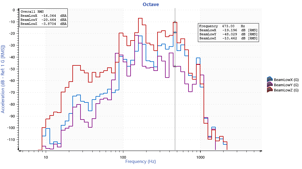
Frequency Weighting and Averaging
The human ear does not perceive changes in sound pressure as loudness because of low sensitivity at low and high frequencies. Engineers apply frequency weighting to filtered acoustic signals to more closely represent the human response to acoustics.
The International Electrotechnical Commission (IEC) developed a standard set of frequency-weighting curves, including A, B, C, and D weights. Many standards include frequency weighting for occupational and environmental noise. The weighting curve selection depends on the type of measurement. For example, the A-weighted curve is ideal when humans are involved with the acoustic signal.
An engineer may also apply averaging to a filtered signal for a more stable representation of the true signal.
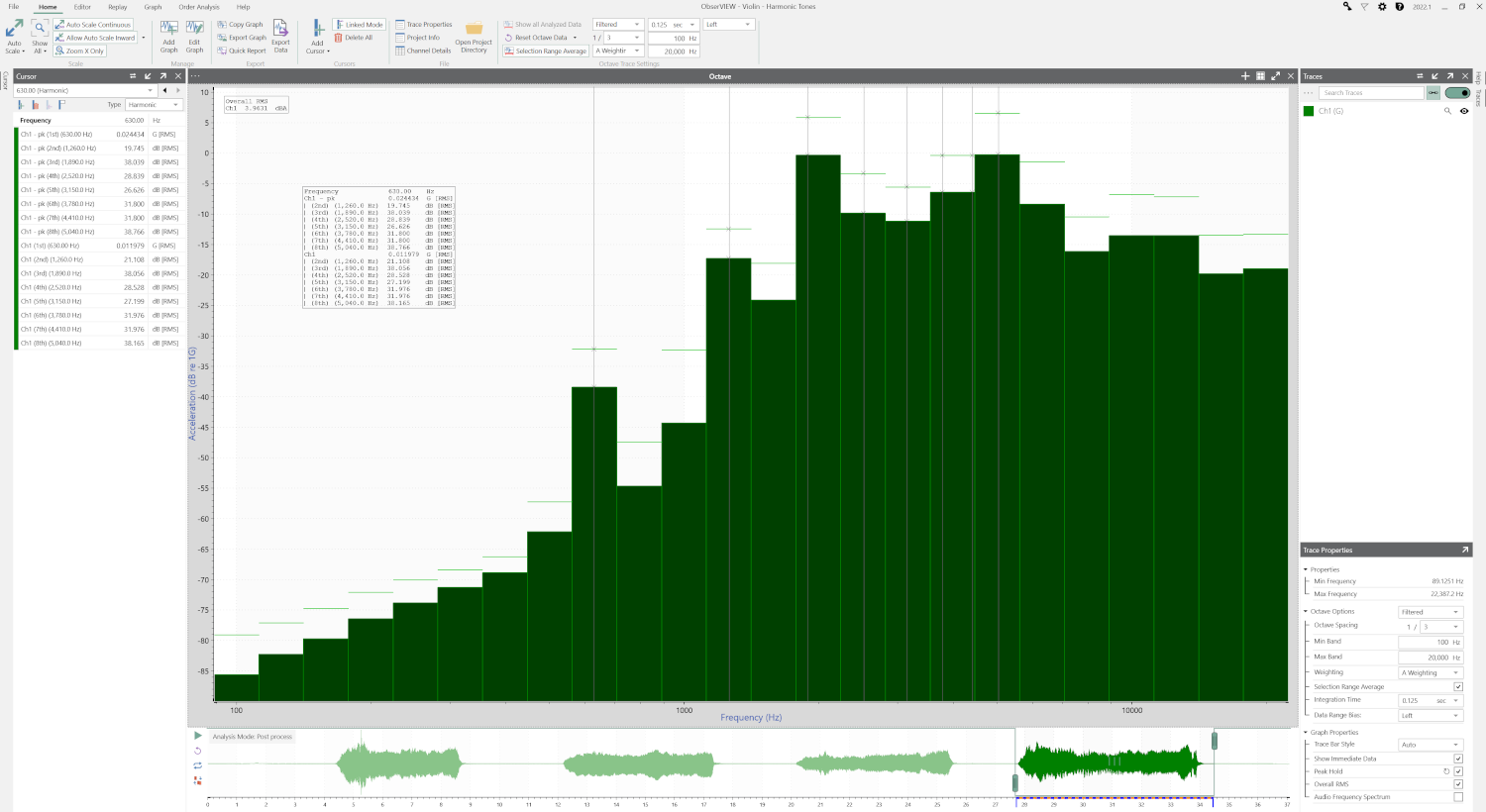
Octave Analysis in ObserVIEW
Octave Analysis Properties in ObserVIEW.
ObserVIEW generates octave band plots with an 8th-order filter to meet IEC 61260-1 Class 1 filter specifications. It includes fast/slow or user-defined time weightings, linear or exponential averaging, and peak hold options. Engineers can also apply A, C, and Z frequency weighting options to meet the IEC 61672-1 requirement.
The software includes the most used fractional octave bands; however, engineers can enter any 1/N fraction that suits their test objectives. ObserVIEW does not have a limit on fractional octave bands. There is a soft limit of 1/96 for computer performance, but the user can override the limit.
The octave band graph supports the advanced functionalities of ObserVIEW, including live analysis, copy-and-paste, and graph traces.
Vibration Research’s data acquisition systems offer the functionality to acquire and analyze acoustic signals. All VR hardware includes a BNC input that supports a microphone and is capable of data acquisition. If a testing lab is already using VR hardware for vibration testing, sound acquisition and analysis is an economical addition.
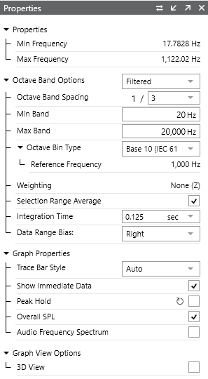
Software Parameters
Overall RMS/SPL
The root mean square (RMS) is a measurement of intensity (amplitude). The ObserVIEW octave band plot splits a signal into bins with octave-spaced center frequencies. The amplitude of each bin represents the signal intensity in that frequency range. The amplitude is calculated as the sum of the range’s RMS values.
The Overall RMS displays the total RMS for the integration period. For pressure units, the measurement is Overall SPL (sound pressure level), which provides the total volume of an audio signal.
Selection Range Average
The selection range average generates the octave band plot using the average amplitude values over a selected data range.
Integration Time
The integration time is the time constant in the exponential moving average, which the software uses to generate the octave bins. For playback, a longer integration time results in slower changes in the plot but less pronounced peaks. In post-processing, the integration time calculates the linear RMS values.
A larger integration time will use a wider time data range to calculate RMS values. The suggested integration times (Fast – 0.125 sec and Slow – 1 sec) are preset values that technicians can use to compare the effects of different integration times. The integration time can also be set manually.
Last updated: February 20, 2024