Introduction
The vibration fatigue of plastics is more complicated than for metals because the effects of strain rate and temperature are more pronounced in plastics. Also, there is a much larger variation in the molecular structures of plastics such that different classes of plastics exhibit different fatigue characteristics. This paper uses the results of experimental fatigue tests on plexiglass (PMMA), ABS, and Polypropylene (PP) to develop a procedure for calculating the Fatigue Damage Spectrum (FDS) for medium high-frequency vibration (50Hz to 500Hz).
BACKGROUND: THE FDS
The Fatigue Damage Spectrum (FDS) [1] measures the relative potential for stresses in the resonant response of structures to cause fatigue failure. For any given resonance frequency the number of cycles to failure is based on the material S-N curve (e.g. Fig. 1). In this study, the range of testing is limited to high cycle fatigue, with the number of cycles, N > 1000, and oscillating peak stress, S, with zero mean. In this range, Basquin [2] proposed an exponential fit to the S-N curve of the form:
|
(1) |
(1) |

where c is a constant and b is the slope of the S-N curve on a log-log plot.
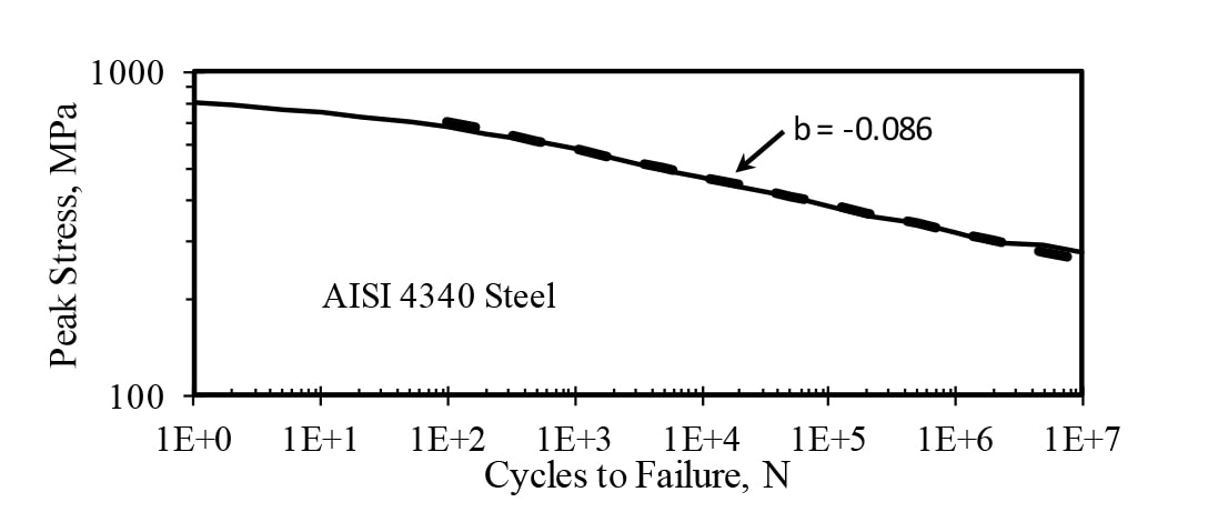
Figure 1. Example of Material S-N Curve with High Cycle Fatigue Curve Fit.
For cases with different stress cycles having different amplitudes, Palmgren [3] and Miner [4] proposed a linear growth of fatigue such that a number of cycles ni at peak stress Si, having Ni as the number of cycles to failure, will produce the fraction ni / Ni of failure. Then, assuming these fractions from different stress loadings can be summed linearly, failure will occur when the sum equals unity or:
|
(2) |
(2) |

For cases where the failure is due to stresses associated with resonance responses in a structure, Lalanne [1] proposed the FDS method for calculating the potential failure using the Palmgren-Miner rule (Eq. 2). Fig. 2 illustrates the response of resonance to random excitation; in this example, the natural frequency, fn = 500Hz.
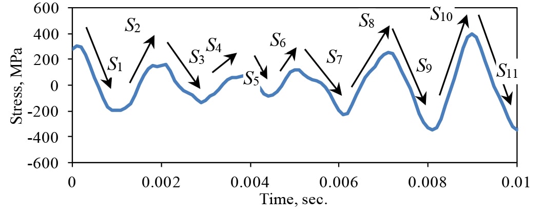
Figure 2. Example of the Response of a Resonance to Random Excitation.
The traverses in stress, S1, S2, etc,. between peaks (max-to-min or min-to max) are considered to be twice the peak stresses of half cycles of cyclic stress. The histogram of these peaks in the stress is computed to form the probability density function (PDF) of the stress peaks, p(S), as illustrated in Fig. 3.
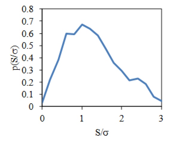
Figure 3. Example of the PDF of the Stress Peaks (Normalized by the Standard Deviation, σ ) of a Randomly Driven Resonance.
To account for the relative damage due to a range of resonance frequencies, fn, the summation in Eq. 2 is converted to an integral over the PDF of stress peaks to compute the Fatigue Damage Spectrum, (FDS):
|
(3) |
(3) |
![\begin{equation*} \text{FDS}=f_{n}t\int^{\infty}_{0}\left[\frac{p(S_{fn})}{(S_{fn}/c)^{1/b}}\right]dS_{fn} \end{equation*}](https://vibrationresearch.com/wp-content/ql-cache/quicklatex.com-e80e98ce8e83a77de31b1a55b98a2989_l3.png "Rendered by QuickLaTeX.com")
The FDS measures relative fatigue damage as a function of frequency.
In most practical cases it is not possible to measure the peak stress levels of resonances, nor are the resonance frequencies known. Therefore, the theoretical response of potential resonances is used to evaluate the FDS. In these cases, the FDS measures the relative fatigue damage a particular excitation will do to potential resonances in the structure.
Hunt [5] showed that the stress, S, in structures vibrating at resonance is proportional to the vibration velocity, Ż,
|
(4) |
(4) |

where ρ is the mass density and E is the elastic modulus of the structural material.
For the case of a random base excitation (as illustrated in Fig. 4) with a specified base acceleration power spectral density, Wa (f), Miles [6] showed that the mean-square vibration response of resonance with a critical damping ratio, ζ, is given by:
|
(5) |
(5) |

where fn is the natural frequency of the resonance.
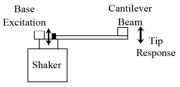
Figure 4. Cantilever Beam Driven by a Base Shaker Excitation with the Tip Vibration Response Measured by an Accelerometer.
Crandall and Mark [7] showed that for a Gaussian random vibration response the PDF of the vibration and stress peaks will have a Rayleigh distribution of the form:
|
(6) |
(6) |

where σ2 is the standard deviation of the stress time history.
Using these theoretical results, Henderson and Piersol [8] derived an expression for the FDS in the case of a random base excitation of a structure. If each resonance response is assumed to have a Gaussian amplitude distribution, then the FDS is given by:
|
(7) |
(7) |
![\begin{equation*} \text{FDS}=c'f_{n}t[W_{a}(f_n)/f_n\zeta]^{-1/2b} \end{equation*}](https://vibrationresearch.com/wp-content/ql-cache/quicklatex.com-23c8a1435418409dd4daddedf1395d5f_l3.png "Rendered by QuickLaTeX.com")
where t is the length of time the structure is exposed to the base excitation and:
|
(8) |
(8) |

where Γ is the Gamma function.
The value of c‘ does not have to be evaluated if the FDS is used as a measure of the relative potential damage a base excitation will cause in structural resonances.
When the vibration excitation is not Gaussian the FDS is computed using the theoretical response of resonances by convolving the excitation with the impulse response of a resonance, h(t) = Ae-2π ζ f t sin (2π f t). The stress response pdf is then evaluated and the FDS is computed by numerically integrating Eq. 3.
PLASTICS
The stress-strain relationship for plastics is more complicated than for metals because of the dependence on temperature and strain rate. In general, plastics are stiffer (with a higher elastic modulus) at lower temperatures and faster strain rates (higher frequencies), and they are softer (with a lower elastic modulus) at higher temperatures and slower strain rates (lower frequencies). Andrews and Tobolsky [9] showed that the temperature and frequency dependencies can be correlated by a temperature shift factor, aT, which is a unique function of temperature for each type of plastic material. A typical example is shown in Fig. 5 [10] where the effective elastic modulus, E, for polypropylene is plotted vs. the reduced frequency, ( aT f ). Also shown is a similar effect on the yield strength of the material.
![Example of the variation of the elastic modulus and yield strength of polypropylene with temperature and frequency [10].](https://vibrationresearch.com/wp-content/uploads/2019/04/FDSforPlastics_Fig5.jpg)
Figure 5. Example of the variation of the elastic modulus and yield strength of polypropylene with temperature and frequency [10].
Theoretically, the scale factor aT is dependent on the activation energy, Ea, and the glass transition temperature, Tg, of the polymer material. This fits well with measured data for amorphous polymers, but not composites. In composites, there are multiple activation energies and the material failure is also dependent on the bonding between components. For this study, only amorphous polymers are considered as a first step in developing an FDS procedure which takes into account the effects of frequency (and temperature).
The simplest mechanical model for amorphous polymers is the Voigt-Maxwell model shown in Fig. 6, where E1 and E2 are elastic moduli, η1 is the relaxation modulus and η2 is the creep modulus. The creep modulus is for very long-term deformation and is ignored here. Then the time-dependent stress-strain (σ-ε) response of the system is:
|
(9) |
(9) |

For sinusoidal motion, ej2π f t, the magnitude of the effective material modulus, Eeff, is (Fig. 7)
|
(10) |
(10) |
![\begin{equation*} |E_{eff}|=E_2\left[\frac{E_{1}^{2}+(2\pi f\eta_1)^2}{(E_1+E_2)^2+(2\pi f\eta_1)^2}\right]^{1/2} \end{equation*}](https://vibrationresearch.com/wp-content/ql-cache/quicklatex.com-2e829d7ac1d615e3a273b4c7da19887c_l3.png "Rendered by QuickLaTeX.com")
At low frequencies, Eeff is equivalent to the two moduli in series. At high frequencies Eeff = E2. The transition occurs at a frequency, f = E1 / (2π η1), which is equivalent to the glass transition temperature Tg in the frequency-temperature scaling.
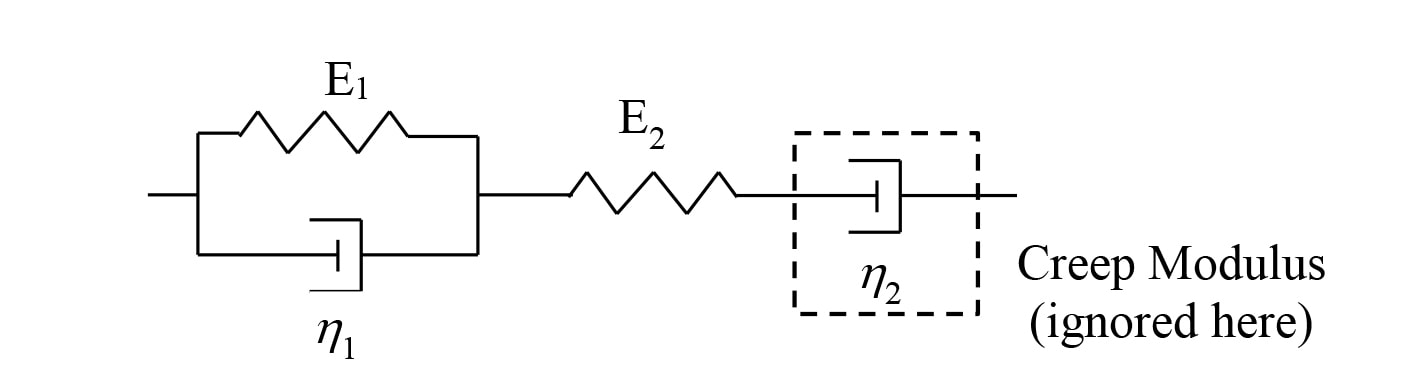
Figure 6. Mechanical Model for the dynamic response of Amorphous Polymers
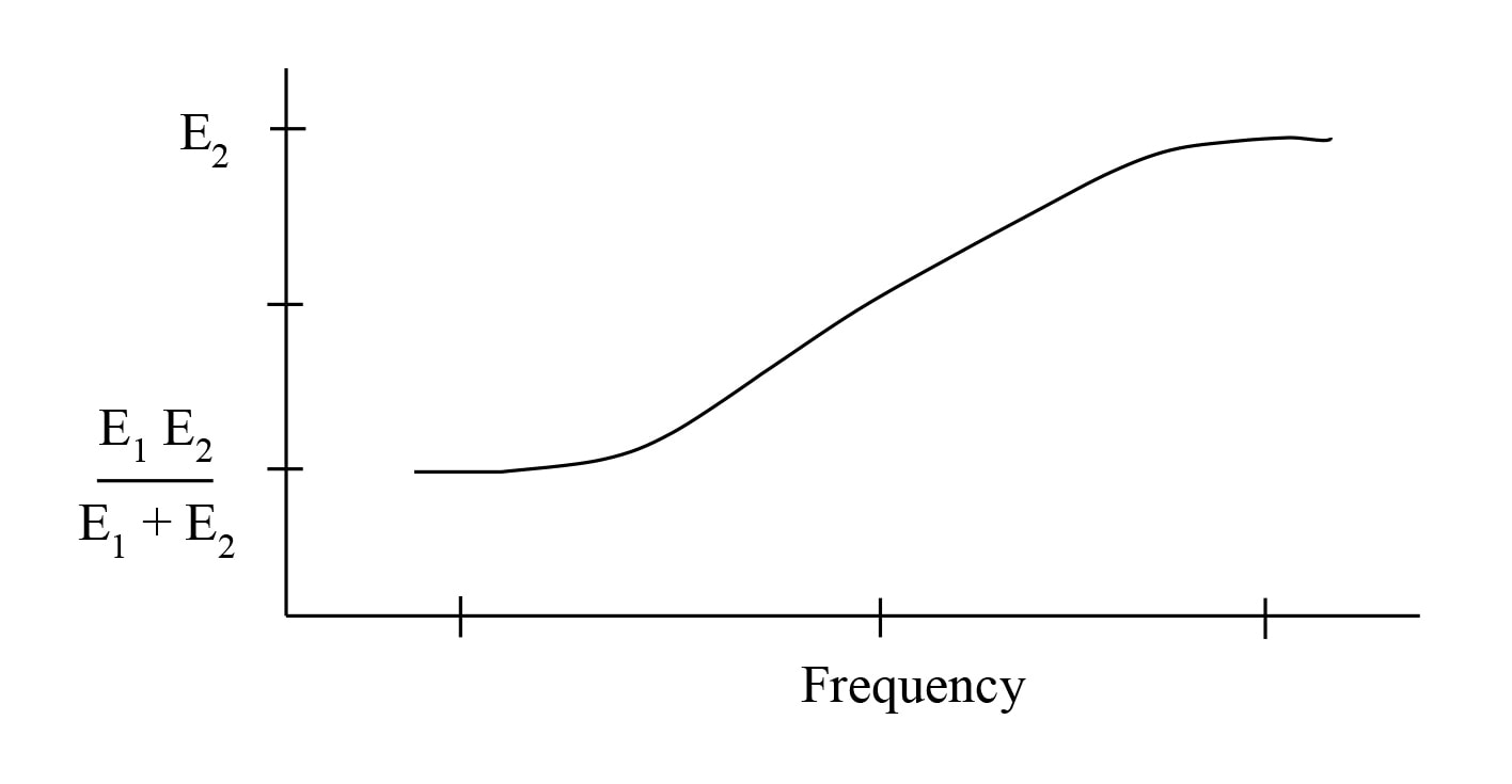
Figure 7. Dynamic Modulus of Amorphous Polymer
As shown in the example of Fig. 5, the tensile strength of the material also increases with frequency, but at a slower rate. This means that the stress for a certain vibration level (Eq. 4) usually increases faster than the failure stress as frequency increases. The easiest way to implement this in the FDS procedure is to modify Eq. 1 to take the form:
|
(11) |
(11) |

where fo is a reference frequency (usually 1Hz) and q is a scaling parameter. The value of q could theoretically be derived from the material properties, but it is usually determined experimentally.
Following the same derivation for the FDS with Gaussian vibration as is done in Eqs. 3 – 8, a formula for the FDS is:
|
(12) |
(12) |
![\begin{align*} \text{FDS}=c'f_n^{1+q/b}t[W_a(f_n)/f_n\zeta]^{-1/2b}\\ c'=\Gamma(1-1/2b)(\rho E/8\pi c^2)^{-1/2b} \end{align*}](https://vibrationresearch.com/wp-content/ql-cache/quicklatex.com-181f1b10e63a04112997bd5c80f4f536_l3.png "Rendered by QuickLaTeX.com")
where Eo is the elastic modulus at the reference frequency. However, the FDS is usually evaluated on a relative basis using experimental and numerical results as illustrated below.
EXPERIMENTAL RESULTS
Experiments have been performed with three plastics (plexiglass: PMMA, polypropylene: PP, and Acrylonitrile Butadiene Styrene: ABS) to validate the modified FDS procedure for plastics outlined above.
First, the S-N curves for a range of resonance frequency excitations are determined using the cantilever beam setup shown in Fig. 4. The thickness, length, and added tip mass are varied to achieve a range of cantilever resonance frequencies. The shaker drives the base sinusoidally at the resonance frequency with a number of amplitudes to achieve a range of stress levels. For each case, the beam is vibrated until it fails. Notches are cut in the beam near the base to achieve a stress concentration of 2 and dictate where the beam failure occurs. Not all beams fail by breaking. An alternate failure is defined by the resonance frequency dropping by 40% (the local stiffness cut in half).
One of the uncertainties is the value of E to use for plastics since the experimental value depends on the strain rate (see Fig. 8). The ASTM standard for tensile testing of plastics specifies a range of 5 to 500mm/min for the stretching rate for a sample with a nominal length of 100mm. Handbooks typically give a range of values for E for plastics. For example, for PP values of E range from 1 to 3GPa. Comparing to the data in Fig. 8, E = 1GPa is approximately the value obtained with a strain rate of 5mm/min. For this study, the lowest value of E given in handbooks is used for consistency and represents the value for low frequencies (0.1 to 1Hz typically).
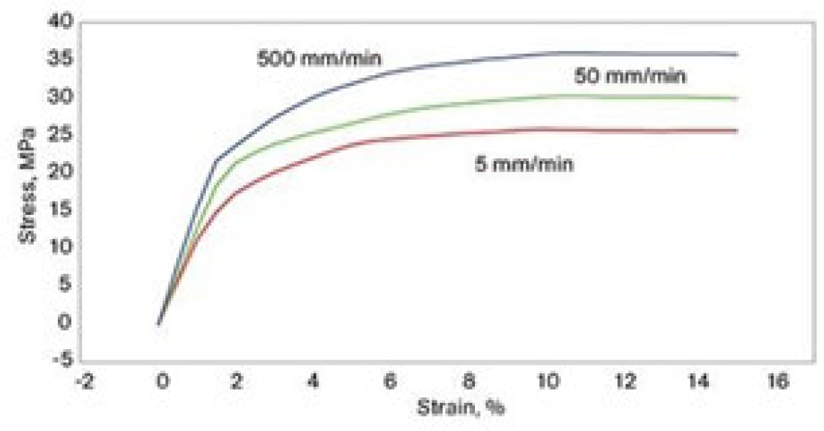
Figure 8. Typical Stress-Strain data for a tensile test of PP with different strain rates.
Fig. 9 shows the fatigue data obtained for PMMA. Since these test samples were manufactured by hand, some of the variability in the data can be attributed to variations in the stress concentration factor. Therefore, these results have not been used further.
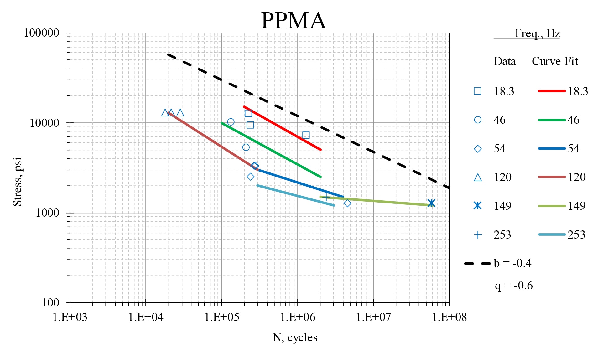
Figure 9. S-N curves for PMMA at different resonance frequencies.
The PP and ABS test samples were manufactured by a CNC milling machine to reduce the variability in the stress concentration factor (designed to be 2.0). Fig. 10 shows the fatigue data for PP. The value for q = log(S1/S2) / log(f1/f2) = -0.4 is obtained from data points at N = 1E6. The dashed line is the theoretical values for 1Hz. Also shown is the nominal yield stress, Sy, for a slow rate tensile test.
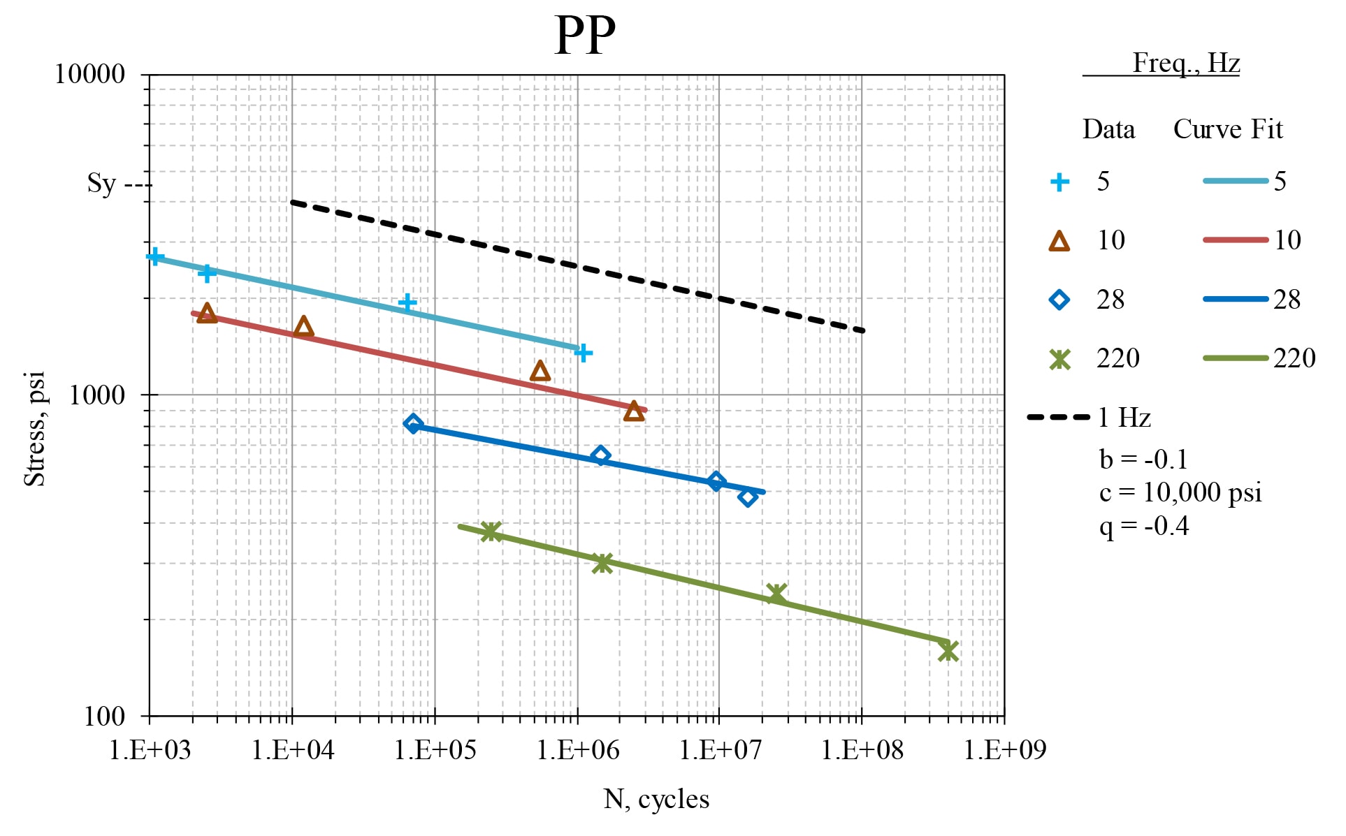
Figure 10. S-N curves for PP at different resonance frequencies.
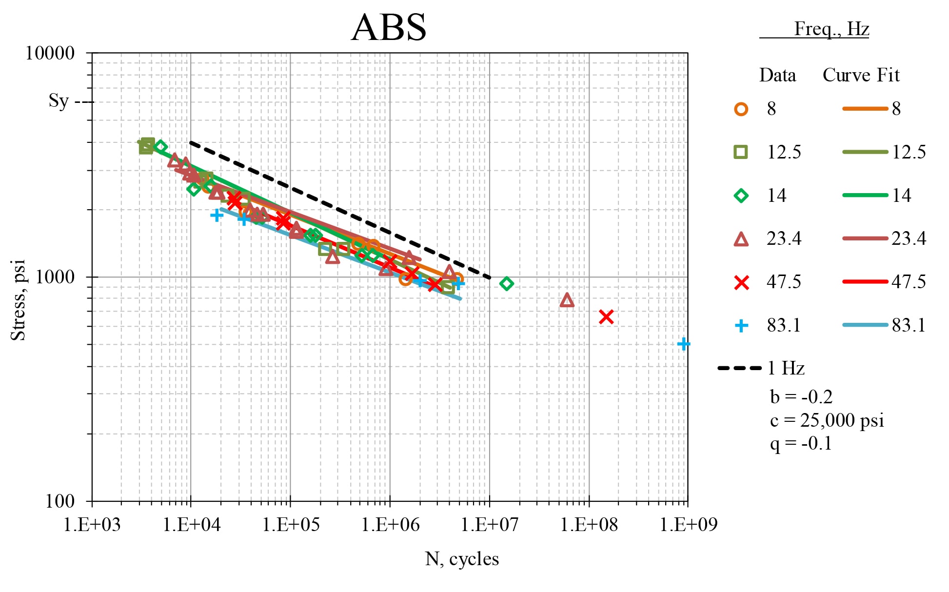
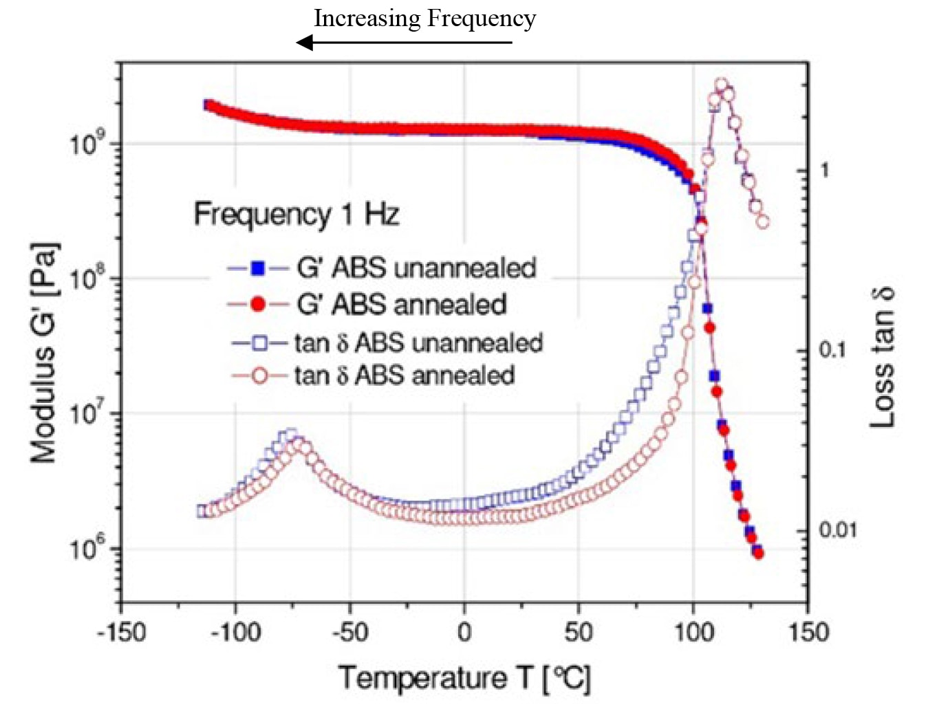
Fig. 11 shows the fatigue data for ABS. The value for q = log(S1/S2) / log(f1/f2) = -0.1 is obtained from data points at N = 1E6. The dashed line is the theoretical values for 1Hz. Also shown is the nominal yield stress, Sy, for a slow rate tensile test. For ABS there is very little frequency dependence. This can also be seen qualitatively in temperature variation data (usually called Dynamic Material Analysis, DMA), where the elastic modulus, E, is measured for a 1Hz excitation while the temperature is varied (see Fig. 12). However, a numerical value of aT, which provides a quantitative temperature-frequency scaling, is very difficult to determine accurately and it is strongly dependent on the material composition. Therefore, it seems best to rely on S-N fatigue tests at different resonance frequencies.
These S-N test results have been applied to the FDS analysis for the PP and ABS cantilever beams. In both cases, a 100mm beam length has been used with thicknesses to give a fundamental resonance of 30Hz. A random base excitation of 0.05G2/Hz with a flat spectrum from 20Hz to 520Hz is used to give an RMS acceleration level of 5.0G. The tip acceleration is measured to be 7.5Grms, giving a damping value of ζ = 0.02.
For PP, a Gaussian excitation of this level would take 5800 hours (240 days) to fail, theoretically. A PP beam has been tested for 48 days without failure. To accelerate the fatigue, a high kurtosis excitation has also been tested. A random base excitation with k = 9 produces a response with k = 5, and numerical evaluation of the FDS predicts a failure at 190 hours. A PP beam has been tested for 230 hours with the damage shown in Fig. 13. The beam has not broken but there is noticeable permanent deformation at the stress concentration resulting in a drop in the resonance frequency by 50%.

Figure 13. Damaged PP test beam.

Figure 14. Damaged ABS test beam.
For ABS, a Gaussian excitation of this level would take 820 hours (34 days) to fail, theoretically. This ABS test beam failed at 28 days. To accelerate the fatigue, a high kurtosis excitation has also been tested. A random base excitation with k = 9 produces a response with k = 5, and numerical evaluation of the FDS predicts a failure at 275 hours. This ABS test beam failed at 250 hours. Both ABS test beams fractured at the stress concentration as shown in Fig. 14.
Further work is needed to extend this analysis to higher frequencies (up to 5000Hz). Also, longer sinusoidal S-N tests need to be performed at various frequencies to determine if there is fatigue limiting stress or a change in the values of b and q for higher values of N and f.